LC Ladder Filter Synthesis via Backpropagation¤

import jax
import jax.numpy as jnp
import matplotlib.pyplot as plt
import numpy as np
import optax

from circulax import compile_circuit, setup_ac_sweep
from circulax.components.electronic import Capacitor, Inductor, Resistor
from circulax.utils import update_params_dict

# Enable 64-bit precision throughout — important for accurate S-parameter
# gradients, especially at high frequencies where small perturbations matter.
jax.config.update("jax_enable_x64", True)

plt.rcParams.update({
    "figure.figsize": (8, 3.5),
    "axes.grid": True,
    "lines.color": "grey",
    "patch.edgecolor": "grey",
    "text.color": "grey",
    "axes.facecolor": "white",
    "axes.edgecolor": "grey",
    "axes.labelcolor": "grey",
    "xtick.color": "grey",
    "ytick.color": "grey",
    "grid.color": "grey",
    "figure.facecolor": "white",
    "figure.edgecolor": "white",
    "savefig.facecolor": "white",
    "savefig.edgecolor": "white",
})

# ── Butterworth prototype parameters ──────────────────────────────────────────
Z0   = 50.0    # reference impedance (Ω)
f_c  = 1e8     # cutoff frequency (Hz) = 100 MHz
wc   = 2 * np.pi * f_c

# N=3 Butterworth g-values: [1, 2, 1]
g1, g2, g3 = 1.0, 2.0, 1.0

L_target = g1 * Z0 / wc          # L1 = L2 (symmetrical T-section)
C_target = g2 / (wc * Z0)        # C1 (shunt)

print(f"Butterworth targets (N=3, Z0={Z0:.0f} Ω, fc={f_c/1e6:.0f} MHz):")
print(f"  L1 = L2 = {L_target*1e9:.4f} nH")
print(f"  C1      = {C_target*1e12:.4f} pF")

# ── Starting values — 3× off from the Butterworth solution ───────────────────
L1_init = 25e-9    # nH  (target: ~79.6 nH)
C1_init = 200e-12  # pF  (target: ~63.7 pF)
L2_init = 25e-9    # nH  (target: ~79.6 nH)

print("\nStarting values:")
print(f"  L1 = {L1_init*1e9:.1f} nH   ({L1_init/L_target:.1f}× target)")
print(f"  C1 = {C1_init*1e12:.1f} pF  ({C1_init/C_target:.1f}× target)")
print(f"  L2 = {L2_init*1e9:.1f} nH   ({L2_init/L_target:.1f}× target)")

# ── Netlist: 3rd-order T-section LC lowpass ───────────────────────────────────
#
#  Rp1,p1 ── L1 ── junction ── L2 ── Rp2,p1
#  (Port1)             │              (Port2)
#                     C1
#                      │
#                     GND
#
# Port nodes are defined by 1 TΩ probe resistors — negligible effect on the
# circuit but they register the node in the port_map.  The Z0=50 Ω source and
# load terminations are injected by setup_ac_sweep, NOT as explicit resistors.
# Including explicit source/load resistors AND letting setup_ac_sweep add Z0
# would give 25 Ω effective termination and the wrong Butterworth values.

net_dict = {
    "instances": {
        "GND":  {"component": "ground"},
        "Rp1":  {"component": "resistor",  "settings": {"R": 1e15}},  # 1 TΩ probe — Port 1
        "L1":   {"component": "inductor",  "settings": {"L": L1_init}},
        "C1":   {"component": "capacitor", "settings": {"C": C1_init}},
        "L2":   {"component": "inductor",  "settings": {"L": L2_init}},
        "Rp2":  {"component": "resistor",  "settings": {"R": 1e15}},  # 1 TΩ probe — Port 2
    },
    "connections": {
        "GND,p1":  ("Rp1,p2", "C1,p2", "Rp2,p2"),
        "Rp1,p1":  "L1,p1",
        "L1,p2":   ("C1,p1", "L2,p1"),
        "L2,p2":   "Rp2,p1",
    },
}

models = {
    "ground":   lambda: 0,
    "resistor": Resistor,
    "inductor":  Inductor,
    "capacitor": Capacitor,
}

circuit = compile_circuit(net_dict, models)
groups = circuit.groups
sys_size = circuit.sys_size
port_map = circuit.port_map

print(f"System size: {sys_size} unknowns")
print(f"Port map: {port_map}")
print(f"\nComponent groups: {list(groups.keys())}")

y_dc = circuit()

# Port 1 = left terminal (input of filter),  Port 2 = right terminal (output)
port_nodes = [port_map["Rp1,p1"], port_map["Rp2,p1"]]
print(f"\nPort node indices: {port_nodes}")

# ── Frequency sweep ───────────────────────────────────────────────────────────
freqs = jnp.logspace(7, 9, 400)   # 10 MHz → 1 GHz (log-spaced)

# ── Analytical Butterworth |S21| target ───────────────────────────────────────
def butterworth_s21(f, fc=f_c, N=3):
    """Ideal N-th order Butterworth |S21| magnitude."""
    return 1.0 / jnp.sqrt(1.0 + (f / fc) ** (2 * N))

target_S21_mag = butterworth_s21(freqs)

# ── Differentiable loss function ──────────────────────────────────────────────
def loss_fn(log_params):
    """MSE between circuit |S21| and Butterworth target, parameterised in log-space."""
    # Recover physical values from log representation
    L1, C1, L2 = jnp.exp(log_params)

    # Functionally update the compiled groups with the new parameter values.
    # update_params_dict(groups, group_name, instance_name, param_key, new_value)
    # uses eqx.tree_at internally — no in-place mutation, fully JAX-traceable.
    g = update_params_dict(groups, "inductor",  "L1", "L", L1)
    g = update_params_dict(g,      "capacitor", "C1", "C", C1)
    g = update_params_dict(g,      "inductor",  "L2", "L", L2)

    # Build and run the AC sweep.  This evaluates F(y) and its Jacobian at
    # y_dc (trivial for a passive circuit), then solves the nodal
    # admittance system at each frequency via jax.vmap.
    run_ac = setup_ac_sweep(g, sys_size, port_nodes, z0=Z0)
    S = run_ac(y_dc, freqs)   # shape: (N_freqs, 2, 2)

    # S21 is the (row=1, col=0) entry: response at port 2 due to excitation at port 1
    S21_mag = jnp.abs(S[:, 1, 0])

    return jnp.mean((S21_mag - target_S21_mag) ** 2)

# Quick sanity check: evaluate the loss at the (wrong) initial parameters
log_params_init = jnp.log(jnp.array([L1_init, C1_init, L2_init]))
loss_init = loss_fn(log_params_init)
print(f"Initial loss: {float(loss_init):.6f}")

# ── Adam optimisation loop ────────────────────────────────────────────────────
#
# We JIT-compile value_and_grad once; subsequent calls reuse the compiled
# computation graph.  The first call includes tracing + compilation overhead;
# from step 2 onward each iteration is fast.

N_STEPS = 300
LR      = 0.05

optimizer = optax.adam(learning_rate=LR)
log_params = jnp.log(jnp.array([L1_init, C1_init, L2_init]))
opt_state  = optimizer.init(log_params)

# Pre-compile the gradient function (tracing happens on the first call)
value_and_grad_fn = jax.jit(jax.value_and_grad(loss_fn))

losses = []
param_history = []  # track [L1, C1, L2] at each step for the convergence plot

for step in range(N_STEPS):
    loss, grads = value_and_grad_fn(log_params)
    losses.append(float(loss))
    param_history.append(np.exp(np.array(log_params)))

    updates, opt_state = optimizer.update(grads, opt_state)
    log_params = optax.apply_updates(log_params, updates)

    if step == 0 or (step + 1) % 50 == 0:
        L1_cur, C1_cur, L2_cur = np.exp(np.array(log_params))
        print(
            f"Step {step+1:3d}: loss={float(loss):.6f}  "
            f"L1={L1_cur*1e9:.2f} nH  "
            f"C1={C1_cur*1e12:.2f} pF  "
            f"L2={L2_cur*1e9:.2f} nH"
        )

# Final recovered values
L1_opt, C1_opt, L2_opt = np.exp(np.array(log_params))

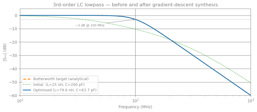
# ── Plot 1: S21 before / after optimisation vs Butterworth target ─────────────

def compute_s21(L1, C1, L2):
    """Evaluate |S21| over the frequency sweep for given component values."""
    g = update_params_dict(groups, "inductor",  "L1", "L", L1)
    g = update_params_dict(g,      "capacitor", "C1", "C", C1)
    g = update_params_dict(g,      "inductor",  "L2", "L", L2)
    run_ac = setup_ac_sweep(g, sys_size, port_nodes, z0=Z0)
    S = jax.jit(run_ac)(y_dc, freqs)
    return np.abs(np.array(S[:, 1, 0]))

S21_init = compute_s21(L1_init, C1_init, L2_init)
S21_opt  = compute_s21(L1_opt,  C1_opt,  L2_opt)
S21_bw   = np.array(target_S21_mag)
freqs_mhz = np.array(freqs) / 1e6

fig, ax = plt.subplots(figsize=(9, 4))

ax.semilogx(freqs_mhz, 20 * np.log10(S21_bw),   color="C1", lw=2,   ls="--", label="Butterworth target (analytical)")
ax.semilogx(freqs_mhz, 20 * np.log10(S21_init),  color="C2", lw=1.5, ls=":",  label=f"Initial  (L={L1_init*1e9:.0f} nH, C={C1_init*1e12:.0f} pF)")
ax.semilogx(freqs_mhz, 20 * np.log10(S21_opt),   color="C0", lw=2,          label=f"Optimised (L={L1_opt*1e9:.1f} nH, C={C1_opt*1e12:.1f} pF)")

# Mark the -3 dB cutoff frequency
ax.axvline(f_c / 1e6, color="grey", ls=":", lw=1, alpha=0.8)
ax.axhline(-3.0,       color="grey", ls=":", lw=1, alpha=0.8)
ax.annotate("−3 dB @ 100 MHz", xy=(f_c/1e6, -3), xytext=(30, -8),
            fontsize=8, color="grey",
            arrowprops=dict(arrowstyle="->", color="grey", lw=0.8))

ax.set_xlabel("Frequency (MHz)")
ax.set_ylabel("|S₂₁| (dB)")
ax.set_title("3rd-order LC lowpass — before and after gradient-descent synthesis")
ax.set_xlim(freqs_mhz[0], freqs_mhz[-1])
ax.set_ylim(-60, 5)
ax.legend(fontsize=9)
plt.tight_layout()
plt.show()

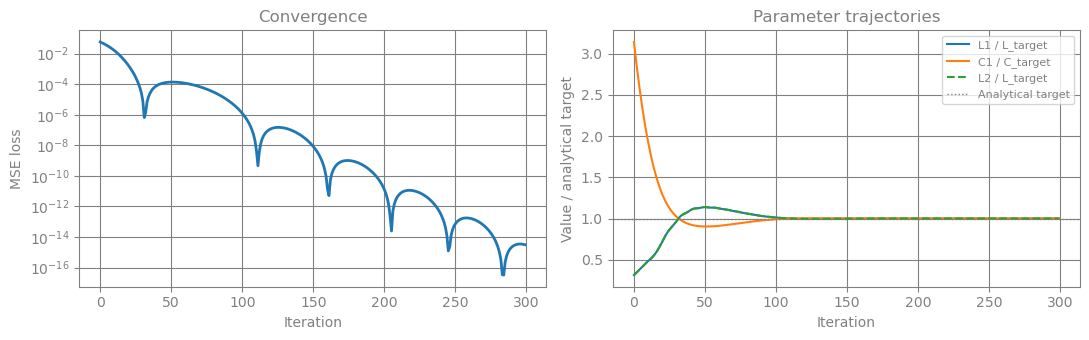
# ── Plot 2: Optimisation convergence ─────────────────────────────────────────

param_history = np.array(param_history)   # shape: (N_STEPS, 3)

fig, (ax1, ax2) = plt.subplots(1, 2, figsize=(11, 3.5))

# Loss curve (log scale)
ax1.semilogy(losses, color="C0", lw=2)
ax1.set_xlabel("Iteration")
ax1.set_ylabel("MSE loss")
ax1.set_title("Convergence")

# Parameter trajectories normalised by target
ax2.plot(param_history[:, 0] / L_target, color="C0", lw=1.5, label="L1 / L_target")
ax2.plot(param_history[:, 1] / C_target, color="C1", lw=1.5, label="C1 / C_target")
ax2.plot(param_history[:, 2] / L_target, color="C2", lw=1.5, ls="--", label="L2 / L_target")
ax2.axhline(1.0, color="grey", ls=":", lw=1, label="Analytical target")
ax2.set_xlabel("Iteration")
ax2.set_ylabel("Value / analytical target")
ax2.set_title("Parameter trajectories")
ax2.legend(fontsize=8)

plt.tight_layout()
plt.show()

# ── Recovered vs analytical values ────────────────────────────────────────────

print("Recovered vs Analytical:")
print(f"  L1: {L1_opt*1e9:.2f} nH  vs  {L_target*1e9:.2f} nH  "
      f"({abs(L1_opt - L_target)/L_target*100:.1f}% error)")
print(f"  C1: {C1_opt*1e12:.2f} pF  vs  {C_target*1e12:.2f} pF  "
      f"({abs(C1_opt - C_target)/C_target*100:.1f}% error)")
print(f"  L2: {L2_opt*1e9:.2f} nH  vs  {L_target*1e9:.2f} nH  "
      f"({abs(L2_opt - L_target)/L_target*100:.1f}% error)")

# Verify passivity of the optimised filter: |S11|² + |S21|² <= 1 at all freqs
g_opt = update_params_dict(groups, "inductor",  "L1", "L", float(L1_opt))
g_opt = update_params_dict(g_opt,  "capacitor", "C1", "C", float(C1_opt))
g_opt = update_params_dict(g_opt,  "inductor",  "L2", "L", float(L2_opt))
run_ac_opt = setup_ac_sweep(g_opt, sys_size, port_nodes, z0=Z0)
S_opt = jax.jit(run_ac_opt)(y_dc, freqs)

power_sum = jnp.abs(S_opt[:, 0, 0])**2 + jnp.abs(S_opt[:, 1, 0])**2
print(f"\nPassivity check: max(|S11|² + |S21|²) = {float(jnp.max(power_sum)):.6f}  (must be ≤ 1.0)")