RF Power Amplifier Optimization via Differentiable Harmonic Balance¤
Inverse design will be used to tune the input and output L-match networks of a 5 GHz Class-A HEMT power amplifier to maximise Power-Added Efficiency (PAE), resulting in the following:
The following is how this is performed in circulax.
Traditional EDA tools (ADS, AWR) solve Harmonic Balance (HB) efficiently, but their built-in optimisers use gradient-free algorithms — genetic algorithms, random search, or Nelder-Mead — that require hundreds of full HB evaluations to converge.
Circulax formulates the HB system as a JAX-differentiable fixed-point problem, which means jax.grad (via Optimistix's ImplicitAdjoint) backpropagates through the HB solver and delivers exact gradients of any scalar figure-of-merit with respect to any circuit parameter — in a single adjoint pass costing roughly one extra forward solve.
In this notebook we: 1. Define a differentiable HEMT model (Curtice-Quadratic with smooth approximations replacing hard if/else branches). 2. Build a 5 GHz power amplifier with input/output L-match networks. 3. Run a Pin sweep to characterise the detuned (initial) amplifier. 4. Use Adam + jax.grad through HB to maximise Power-Added Efficiency (PAE) by tuning the four matching-network L/C values — obtaining analytic gradients at each step.
import jax
import jax.nn as jnn
import jax.numpy as jnp
import numpy as np
import optax
import plotly.graph_objects as go
import plotly.io as pio
from plotly.subplots import make_subplots

from circulax import compile_circuit
from circulax.components.base_component import component
from circulax.components.electronic import (
    Capacitor,
    Inductor,
    Resistor,
    VoltageSource,
    VoltageSourceAC,
)

jax.config.update("jax_enable_x64", True)

pio.templates.default = "plotly_white"
pio.renderers.default = "png"
print("JAX backend:", jax.default_backend())
JAX backend: cpu
Phase 1 — Differentiable HEMT Model¤
Standard SPICE transistor models use piecewise branching:
if Vgs < Vp:
    Ids = 0          # pinch-off
elif Vds < Vgs - Vp:
    Ids = quadratic  # linear region
else:
    Ids = saturated  # saturation region
Python if/else on traced JAX values breaks the Jacobian: the derivative is either zero or undefined at the transition. The fix is smooth approximations:
| Hard branch | Smooth replacement | Why |
|---|---|---|
max(0, Vgs - Vp) | softplus(Vgs - Vp) | Differentiable everywhere |
| Hard saturation clamp | tanh(α Vds) | Smooth S-curve, saturates as Vds → ∞ |
| Abrupt Qgs step | softplus integral | Continuous dQgs/dVgs (transcapacitance) |
The model is a Modified Curtice-Quadratic with three-terminal gate/drain/source ports.
@component(ports=("g", "d", "s"))
def HEMT(signals, s,
         beta=0.012, Vp=-2.0, lam=0.05, alpha=4.0,
         Cgs0=0.3e-12, Cgs1=0.1e-12, Cgd0=0.05e-12):
    # Modified Curtice-Quadratic HEMT with smooth approximations.
    #
    # Parameters
    # ----------
    # beta  : transconductance parameter (A/V^2)
    # Vp    : pinch-off voltage (V)
    # lam   : channel-length modulation (1/V)
    # alpha : saturation slope (1/V)
    # Cgs0  : linear gate-source capacitance (F)
    # Cgs1  : nonlinear gate-source capacitance coefficient (F)
    # Cgd0  : gate-drain (Miller) capacitance (F)
    Vgs = signals.g - signals.s
    Vds = signals.d - signals.s
    Vgd = signals.g - signals.d

    sp_scale = 10.0
    # Smooth pinch-off: softplus replaces max(0, Vgs - Vp)
    sp = jnn.softplus(sp_scale * (Vgs - Vp)) / sp_scale

    # Drain current: quadratic in pinch-off voltage, tanh saturation
    Ids = beta * sp**2 * (1.0 + lam * Vds) * jnp.tanh(alpha * Vds)

    # Gate-source charge: integral of sigmoid = softplus (differentiable everywhere)
    Qgs = Cgs0 * Vgs + Cgs1 * jnn.softplus(sp_scale * (Vgs - Vp)) / sp_scale
    # Gate-drain (Miller) charge: linear
    Qgd = Cgd0 * Vgd

    f = {"g": 0.0,   "d": Ids,  "s": -Ids}
    q = {"g": Qgs + Qgd, "d": -Qgd, "s": -Qgs}
    return f, q


# ── Smoke test ────────────────────────────────────────────────────────────────────────────────
hemt_test = HEMT()
f, q = hemt_test(g=0.0, d=3.0, s=0.0)
print(f"Ids at Vgs=0 V,   Vds=3 V: {f['d']*1e3:.2f} mA  (Idss)")

f2, _ = hemt_test(g=-2.5, d=3.0, s=0.0)
print(f"Ids at Vgs=-2.5 V (below pinch-off): {f2['d']*1e6:.3f} µA  (should be ~0)")

# Verify JAX-differentiability
gm = float(jax.grad(lambda vg: hemt_test(g=vg, d=3.0, s=0.0)[0]["d"])(0.0))
print(f"gm at Vgs=0, Vds=3 V: {gm*1e3:.2f} mS")
Ids at Vgs=0 V,   Vds=3 V: 55.20 mA  (Idss)
Ids at Vgs=-2.5 V (below pinch-off): 0.006 µA  (should be ~0)


gm at Vgs=0, Vds=3 V: 55.20 mS
def compute_Ids(Vgs, Vds,
               beta=0.012, Vp=-2.0, lam=0.05, alpha=4.0):
    sp_scale = 10.0
    sp = jnn.softplus(sp_scale * (Vgs - Vp)) / sp_scale
    return beta * sp**2 * (1.0 + lam * Vds) * jnp.tanh(alpha * Vds)


Vds_arr = jnp.linspace(0.0, 5.0, 200)
Vgs_arr = jnp.linspace(-3.0, 0.5, 200)

fig = make_subplots(
    rows=1, cols=2,
    subplot_titles=("Output Characteristics", "Transconductance vs Vgs  (Vds = 3 V)"),
)

# Left: Output characteristics
colors_iv = ["#1f77b4", "#ff7f0e", "#2ca02c", "#d62728"]
for Vgs_val, col in zip([-1.5, -1.0, -0.5, 0.0], colors_iv):
    ids_curve = jax.vmap(lambda vds: compute_Ids(Vgs_val, vds))(Vds_arr)
    fig.add_trace(
        go.Scatter(
            x=np.array(Vds_arr),
            y=np.array(ids_curve) * 1e3,
            mode="lines",
            name=f"Vgs = {Vgs_val} V",
            line=dict(color=col),
        ),
        row=1, col=1,
    )
# Vertical bias line
fig.add_vline(x=3.0, line=dict(color="grey", width=1, dash="dash"),
              annotation_text="Vds = 3 V (bias)", annotation_position="top right",
              row=1, col=1)

# Right: Transconductance
ids_vgs = jax.vmap(lambda vgs: compute_Ids(vgs, 3.0))(Vgs_arr)
gm = jnp.gradient(ids_vgs, Vgs_arr)
fig.add_trace(
    go.Scatter(
        x=np.array(Vgs_arr),
        y=np.array(gm) * 1e3,
        mode="lines",
        name="gm (mS)",
        line=dict(color="#ff7f0e", width=2),
        showlegend=True,
    ),
    row=1, col=2,
)
fig.add_vline(x=-0.5, line=dict(color="#1f77b4", width=1.5, dash="dash"),
              annotation_text="Vgg = −0.5 V (bias)", annotation_position="top right",
              row=1, col=2)

fig.update_xaxes(title_text="Vds (V)", row=1, col=1)
fig.update_yaxes(title_text="Ids (mA)", row=1, col=1)
fig.update_xaxes(title_text="Vgs (V)", row=1, col=2)
fig.update_yaxes(title_text="gm (mS)", row=1, col=2)
fig.update_layout(margin=dict(t=80, b=60, l=60, r=60), height=400, width=900, legend=dict(tracegroupgap=0))
fig.show()
print("No kinks or discontinuities → Jacobian is well-defined everywhere.")
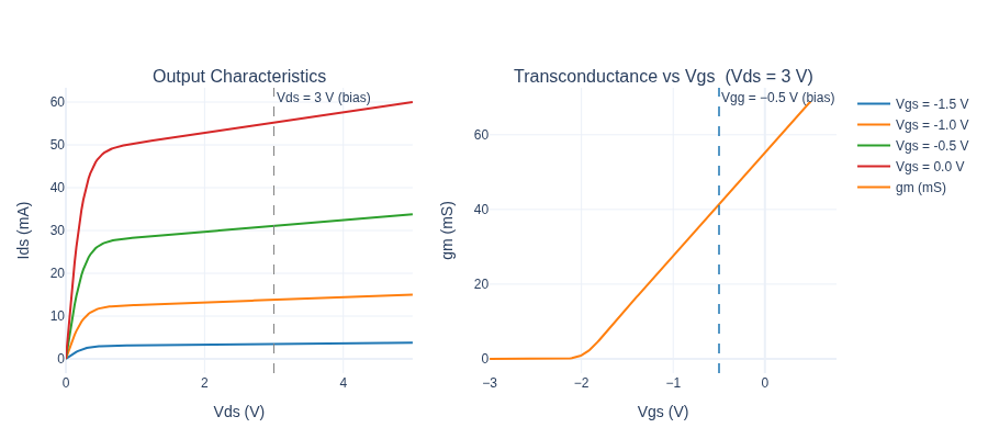
No kinks or discontinuities → Jacobian is well-defined everywhere.
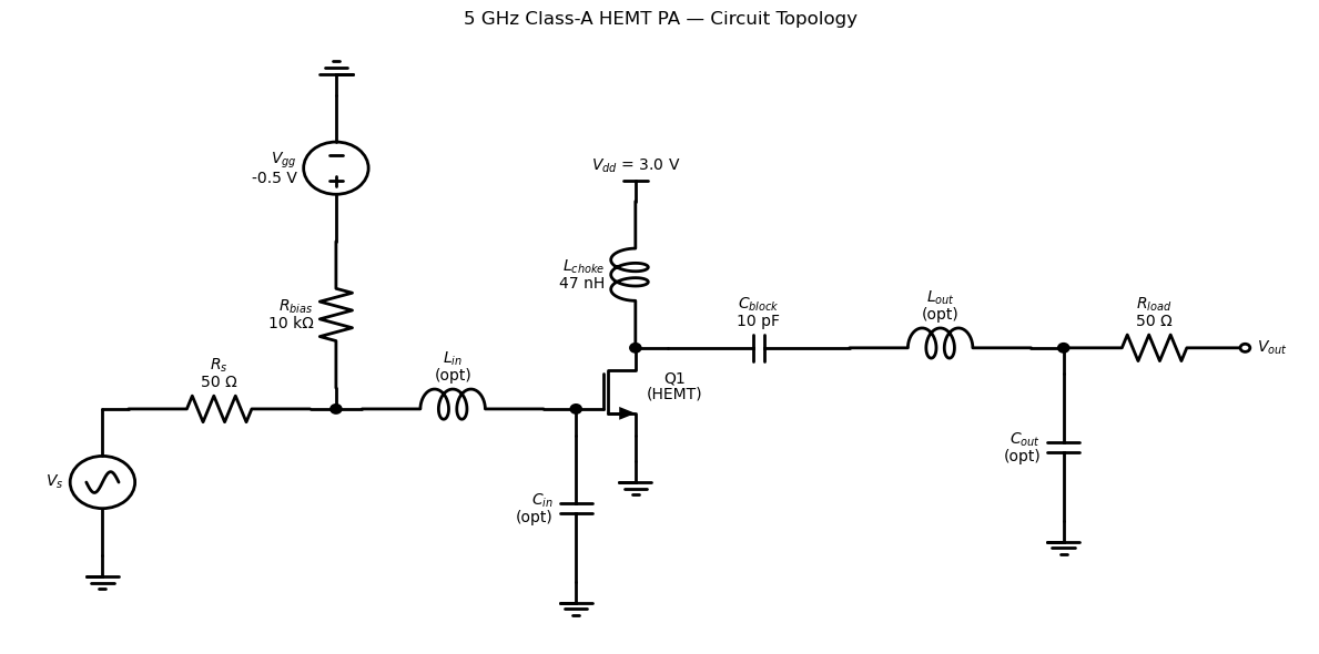
Phase 2 — PA Circuit Architecture¤
Component roles:
| Component | Value | Purpose |
|---|---|---|
Rs_src | 50 Ω | Source impedance |
R_bias | 10 kΩ | Gate bias resistor (high RF impedance) |
L_choke | 47 nH | RF choke: Z = 1.5 kΩ at 5 GHz → DC path to Vdd, RF open |
C_block | 10 pF | DC block: Z = 3.2 Ω at 5 GHz → RF short, blocks Vdd from output |
L_in, C_in | optimised | Input L-match: transforms 50 Ω source → Zin* at gate |
L_out, C_out | optimised | Output L-match: transforms Ropt at drain → 50 Ω load |
R_load | 50 Ω | Load resistance |
The optimal load resistance for maximum class-A output power is Ropt ≈ (Vdd − Vknee) / (2 Idq). The matching networks are initialised deliberately off-resonance; the optimizer will tune them.
# ── Frequency and harmonic parameters ──────────────────────────────────────────────
F0      = 5e9    # Hz  (5 GHz)
N_HARM  = 7      # harmonics → K = 15 time points per period
K       = 2 * N_HARM + 1

# ── Bias and HEMT parameters ───────────────────────────────────────────────────
Vgg_val     = -0.5   # V  gate bias
Vdd_val     =  3.0   # V  drain supply
hemt_params = dict(beta=0.012, Vp=-2.0, lam=0.05, alpha=4.0,
                   Cgs0=0.3e-12, Cgs1=0.1e-12, Cgd0=0.05e-12)

# ── Matching network — deliberately detuned starting values ───────────────────────────
L_in_init  = 0.3e-9;  C_in_init  = 0.5e-12   # input L-match
L_out_init = 0.3e-9;  C_out_init = 0.5e-12   # output L-match

# ── Fixed bias tee values (not optimised) ─────────────────────────────────────────────────
L_choke_val = 47e-9   # 47 nH → Z ≈ 1.5 kΩ at 5 GHz  (RF open)
C_block_val = 10e-12  # 10 pF → Z ≈ 3.2 Ω at 5 GHz   (RF short)
R_bias_val  = 10e3    # 10 kΩ (gate bias, high RF impedance)

V_in_init   = 0.1    # V amplitude for initial compile

# ── SAX-format netlist ────────────────────────────────────────────────────────────────────
pa_net = {
    "instances": {
        "Vs":      {"component": "voltagesourceac", "settings": {"V": V_in_init, "freq": F0}},
        "Rs_src":  {"component": "resistor",        "settings": {"R": 50.0}},
        "L_in":    {"component": "inductor",        "settings": {"L": L_in_init}},
        "C_in":    {"component": "capacitor",       "settings": {"C": C_in_init}},
        "R_bias":  {"component": "resistor",        "settings": {"R": R_bias_val}},
        "Vgg":     {"component": "voltagesource",   "settings": {"V": Vgg_val}},
        "Q1":      {"component": "hemt",            "settings": hemt_params},
        "L_choke": {"component": "inductor",        "settings": {"L": L_choke_val}},
        "Vdd":     {"component": "voltagesource",   "settings": {"V": Vdd_val}},
        "C_block": {"component": "capacitor",       "settings": {"C": C_block_val}},
        "L_out":   {"component": "inductor",        "settings": {"L": L_out_init}},
        "C_out":   {"component": "capacitor",       "settings": {"C": C_out_init}},
        "R_load":  {"component": "resistor",        "settings": {"R": 50.0}},
        "GND":     {"component": "ground"},
    },
    "connections": {
        "Vs,p1":      "Rs_src,p1",
        "Vs,p2":      "GND,p1",
        "Rs_src,p2":  "L_in,p1",
        "L_in,p2":    ("Q1,g", "C_in,p1", "R_bias,p1"),
        "C_in,p2":    "GND,p1",
        "R_bias,p2":  "Vgg,p1",
        "Vgg,p2":     "GND,p1",
        "Q1,s":       "GND,p1",
        "Q1,d":       ("L_choke,p2", "C_block,p1"),
        "L_choke,p1": "Vdd,p1",
        "Vdd,p2":     "GND,p1",
        "C_block,p2": "L_out,p1",
        "L_out,p2":   ("C_out,p1", "R_load,p1"),
        "C_out,p2":   "GND,p1",
        "R_load,p2":  "GND,p1",
    },
    "ports": {"gate": "Q1,g", "drain": "Q1,d", "load": "R_load,p1"},
}

models = {
    "voltagesourceac": VoltageSourceAC,
    "voltagesource":   VoltageSource,
    "resistor":        Resistor,
    "inductor":        Inductor,
    "capacitor":       Capacitor,
    "hemt":            HEMT,
    "ground":          lambda: 0,
}

circuit = compile_circuit(pa_net, models, backend="dense")
print(f"System size : {circuit.sys_size} unknowns")
print(f"Named ports : {list(pa_net['ports'])}")

# Internal state used for drain-current and DC-power inspection.
choke_iL_idx = circuit.port_map["L_choke,i_L"]
print(f"Internal L_choke current state index: {choke_iL_idx}")


def _pa_params(V_in=None, L_in=None, C_in=None, L_out=None, C_out=None):
    updates = {}
    if V_in is not None:
        updates["Vs.V"] = V_in
    if L_in is not None:
        updates["L_in.L"] = L_in
    if C_in is not None:
        updates["C_in.C"] = C_in
    if L_out is not None:
        updates["L_out.L"] = L_out
    if C_out is not None:
        updates["C_out.C"] = C_out
    return updates


def _run_pa_hb(params, y_flat_init=None):
    return circuit.hb(
        freq=F0,
        harmonics=N_HARM,
        y0=y_dc,
        params=params,
        y_flat_init=y_flat_init,
    )
System size : 15 unknowns
Named ports : ['gate', 'drain', 'load']
Internal L_choke current state index: 9
y_dc = circuit.dc()

V_gate     = float(circuit.port(y_dc, "gate"))
V_drain    = float(circuit.port(y_dc, "drain"))
I_drain_dc = float(y_dc[choke_iL_idx])

# Verify with HEMT formula
sp_scale = 10.0
Vp = -2.0; beta = 0.012; alpha = 4.0; lam = 0.05
sp = float(jnn.softplus(sp_scale * (V_gate - Vp)) / sp_scale)
Ids_check = beta * sp**2 * (1 + lam * V_drain) * float(jnp.tanh(alpha * V_drain))

print("DC Operating Point")
print(f"  V_gate  = {V_gate:.4f} V   (Vgg = {Vgg_val} V)")
print(f"  V_drain = {V_drain:.4f} V   (Vdd = {Vdd_val} V)")
print(f"  I_drain = {I_drain_dc*1e3:.2f} mA  (from L_choke inductor state)")
print(f"  Ids check = {Ids_check*1e3:.2f} mA  (from HEMT formula directly)")
print(f"  Pdc     = {Vdd_val * I_drain_dc * 1e3:.1f} mW")

Ropt = (Vdd_val - 0.3) / (2 * I_drain_dc) if I_drain_dc > 1e-6 else float("inf")
print("\n  Ropt ≈ (Vdd - Vknee) / (2 Idq)")
print(f"       = ({Vdd_val} - 0.3) / (2 × {I_drain_dc*1e3:.1f} mA)")
print(f"       = {Ropt:.1f} Ω  (optimal load for class-A max power)")
print(f"\n  The output L-match must transform 50 Ω → {Ropt:.0f} Ω at 5 GHz.")
DC Operating Point
  V_gate  = -0.0025 V   (Vgg = -0.5 V)
  V_drain = 3.0000 V   (Vdd = 3.0 V)
  I_drain = 55.06 mA  (from L_choke inductor state)
  Ids check = 55.06 mA  (from HEMT formula directly)
  Pdc     = 165.2 mW

  Ropt ≈ (Vdd - Vknee) / (2 Idq)
       = (3.0 - 0.3) / (2 × 55.1 mA)
       = 24.5 Ω  (optimal load for class-A max power)

  The output L-match must transform 50 Ω → 25 Ω at 5 GHz.
Phase 2 — Forward PA Simulation via Harmonic Balance¤
How Harmonic Balance works here:
The HB solver represents the periodic steady-state as K = 2N+1 = 15 equally-spaced time samples per period (T = 200 ps at 5 GHz), or equivalently as the DC component plus N = 7 complex Fourier coefficients.
At each Newton iteration the solver evaluates the DAE residual F(y) + dQ/dt = 0 in the frequency domain by: 1. IDFT the frequency-domain unknowns to the time domain. 2. Evaluate all component nonlinearities (HEMT etc.) at each of the K time points. 3. DFT back to frequency domain and assemble the residual.
The Jacobian is assembled analytically (via jax.jacfwd) and the system is solved with a dense LU factorisation.
Warm-starting: For a driven PA (not an oscillator), the source always forces a non-trivial periodic response. Tiling the DC solution y_dc across K time steps is a reliable warm start.
# compute_powers: differentiable PA metrics from HB Fourier coefficients.
# y_freq[k, node] is the normalised complex Fourier coefficient at harmonic k.
# The time-domain peak amplitude is  2 * |y_freq[k, node]|  for k >= 1.
def compute_powers(y_freq, V_src_amp, Vdd):
    # Output power at fundamental
    V_load_amp = 2.0 * jnp.abs(circuit.port(y_freq, "load")[1])
    Pout_W     = V_load_amp**2 / (4.0 * 50.0)   # delivered to matched 50 Ω

    # Available input power
    Pin_W = V_src_amp**2 / (8.0 * 50.0)

    # DC power: Vdd × mean drain current  (DC harmonic = y_freq[0])
    I_dc  = jnp.real(y_freq[0, choke_iL_idx])
    Pdc_W = Vdd * I_dc

    PAE      = (Pout_W - Pin_W) / (Pdc_W + 1e-20)
    Pout_dBm = 10.0 * jnp.log10(Pout_W / 1e-3 + 1e-20)
    Pin_dBm  = 10.0 * jnp.log10(Pin_W  / 1e-3 + 1e-20)
    Gain_dB  = Pout_dBm - Pin_dBm
    return Pout_dBm, Gain_dB, PAE


# ── Single-point verification at +10 dBm available input ─────────────────────────
V_test = float(jnp.sqrt(8.0 * 50.0 * 10.0 ** (10.0 / 10.0) * 1e-3))
print(f"Test point: +10 dBm available input → V_amplitude = {V_test:.3f} V")

y_flat_init = jnp.tile(y_dc, K)
y_time_ref, y_freq_ref = _run_pa_hb(_pa_params(V_in=V_test), y_flat_init=y_flat_init)

Pout_t, Gain_t, PAE_t = compute_powers(y_freq_ref, V_test, Vdd_val)
print(f"\n  Pout = {float(Pout_t):.1f} dBm")
print(f"  Gain = {float(Gain_t):.1f} dB")
print(f"  PAE  = {float(PAE_t)*100:.1f}%")

drain_ref = circuit.port(y_freq_ref, "drain")
gate_ref = circuit.port(y_freq_ref, "gate")
print(f"\n  Drain voltage swing : {float(2*jnp.abs(drain_ref[1])):.3f} V peak")
print(f"  Gate voltage swing  : {float(2*jnp.abs(gate_ref[1])):.3f} V peak")
h3_ratio = float(jnp.abs(drain_ref[3]) / (jnp.abs(drain_ref[1]) + 1e-20))
print(f"  3rd harmonic at drain: {float(2*jnp.abs(drain_ref[3]))*1e3:.1f} mV  ({h3_ratio*100:.1f}% of fundamental)")
Test point: +10 dBm available input → V_amplitude = 2.000 V


  Pout = 13.7 dBm
  Gain = 3.7 dB
  PAE  = 7.3%

  Drain voltage swing : 1.974 V peak
  Gate voltage swing  : 1.111 V peak
  3rd harmonic at drain: 6.4 mV  (0.3% of fundamental)
Pin_dBm_vals = np.linspace(-10, 22, 17)
V_amp_vals   = np.sqrt(8.0 * 50.0 * 10.0 ** (Pin_dBm_vals / 10.0) * 1e-3)


def run_at_amplitude(V_in: jax.Array):
    # Run HB and return (Pout_dBm, Gain_dB, PAE) at source amplitude V_in.
    _, y_freq_i = _run_pa_hb(_pa_params(V_in=V_in), y_flat_init=jnp.tile(y_dc, K))
    return compute_powers(y_freq_i, V_in, Vdd_val)


run_at_amplitude_jit = jax.jit(run_at_amplitude)

Pout_list, Gain_list, PAE_list = [], [], []
print("Pin sweep (detuned matching network):")
print(f"{'Pin (dBm)':>12}  {'Pout (dBm)':>12}  {'Gain (dB)':>10}  {'PAE (%)':>8}")
print("-" * 50)
for Pin_dBm, V_in in zip(Pin_dBm_vals, V_amp_vals):
    Pout, Gain, PAE = run_at_amplitude_jit(jnp.array(V_in))
    Pout_list.append(float(Pout))
    Gain_list.append(float(Gain))
    PAE_list.append(float(PAE) * 100)
    if round(Pin_dBm) in (-10, -2, 6, 14, 22):
        print(f"{Pin_dBm:>12.0f}  {float(Pout):>12.1f}  {float(Gain):>10.1f}  {float(PAE)*100:>8.1f}")
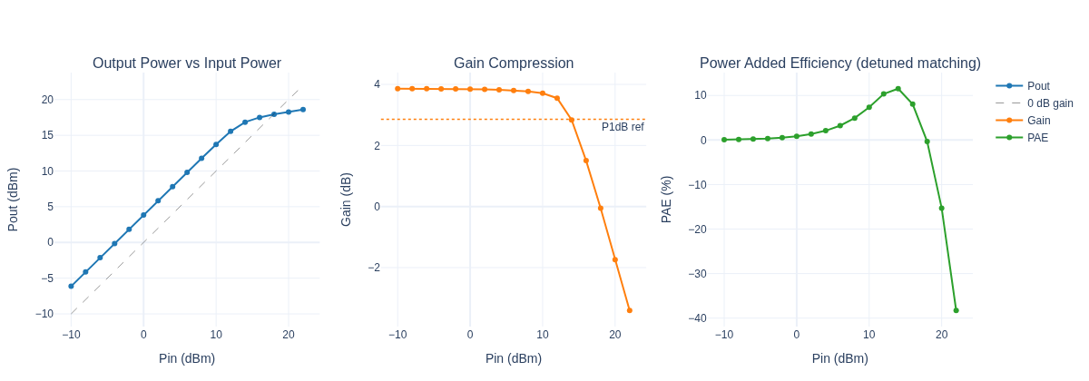
Pin sweep (detuned matching network):
   Pin (dBm)    Pout (dBm)   Gain (dB)   PAE (%)
--------------------------------------------------


         -10          -6.1         3.9       0.1
          -2           1.9         3.9       0.5
           6           9.8         3.8       3.2
          14          16.8         2.8      11.5
          22          18.6        -3.4     -38.3
fig = make_subplots(
    rows=1, cols=3,
    subplot_titles=("Output Power vs Input Power", "Gain Compression", "Power Added Efficiency (detuned matching)"),
)

# Pout vs Pin
fig.add_trace(
    go.Scatter(x=list(Pin_dBm_vals), y=Pout_list, mode="lines+markers",
               name="Pout", marker=dict(size=6), line=dict(color="#1f77b4", width=2)),
    row=1, col=1,
)
fig.add_trace(
    go.Scatter(x=list(Pin_dBm_vals), y=list(Pin_dBm_vals), mode="lines",
               name="0 dB gain", line=dict(color="black", width=1, dash="dash"), opacity=0.4),
    row=1, col=1,
)

# Gain vs Pin
fig.add_trace(
    go.Scatter(x=list(Pin_dBm_vals), y=Gain_list, mode="lines+markers",
               name="Gain", marker=dict(size=6), line=dict(color="#ff7f0e", width=2)),
    row=1, col=2,
)
if Gain_list:
    p1db_ref = Gain_list[0] - 1
    fig.add_hline(y=p1db_ref, line=dict(color="#ff7f0e", width=1.5, dash="dot"),
                  annotation_text="P1dB ref", annotation_position="bottom right",
                  row=1, col=2)

# PAE vs Pin
fig.add_trace(
    go.Scatter(x=list(Pin_dBm_vals), y=PAE_list, mode="lines+markers",
               name="PAE", marker=dict(size=6), line=dict(color="#2ca02c", width=2)),
    row=1, col=3,
)

fig.update_xaxes(title_text="Pin (dBm)", row=1, col=1)
fig.update_yaxes(title_text="Pout (dBm)", row=1, col=1)
fig.update_xaxes(title_text="Pin (dBm)", row=1, col=2)
fig.update_yaxes(title_text="Gain (dB)", row=1, col=2)
fig.update_xaxes(title_text="Pin (dBm)", row=1, col=3)
fig.update_yaxes(title_text="PAE (%)", rangemode="tozero", row=1, col=3)

fig.update_layout(margin=dict(t=80, b=60, l=60, r=60), height=420, width=1200)
fig.show()
Phase 3 — Gradient-Based Matching Network Optimisation¤
Why matching matters for PAE:
PAE is maximised when the drain sees the optimal load resistance Ropt ≈ (Vdd − Vknee) / (2 Idq). With the detuned L-match, the effective load at 5 GHz differs from Ropt — power is reflected rather than delivered. The input match is similarly off, so extra drive power is wasted.
Gradient flow through Harmonic Balance:
loss = −PAE(L_in, C_in, L_out, C_out) where PAE is computed from the HB fixed point. Circulax uses Optimistix's ImplicitAdjoint to differentiate through the Newton solver:
This costs one extra linear solve per gradient evaluation (the adjoint), regardless of how many Newton iterations the forward solve needed. Compare that to finite differences: 2 × n_params extra HB solves.
Parameterisation: We optimise log(L) and log(C) so that the physical values remain positive and cover several decades without constraint handling.
# ── Target: maximise PAE at +12 dBm input (moderate saturation) ─────────────────────
V_target = float(jnp.sqrt(8.0 * 50.0 * 10.0 ** (12.0 / 10.0) * 1e-3))
print(f"Optimisation target: Pin = +12 dBm  (V_source amplitude = {V_target:.3f} V)")

# Fixed warm start: tile DC solution across K time points.
# For a driven PA the source always forces a non-trivial solution, so this is reliable.
y_flat_warmstart = jnp.tile(y_dc, K)


def loss_fn(log_params: jax.Array) -> jax.Array:
    # Negative PAE - minimising this maximises PAE at +12 dBm input.
    L_in, C_in, L_out, C_out = jnp.exp(log_params)

    _, y_freq_i = _run_pa_hb(
        _pa_params(V_in=V_target, L_in=L_in, C_in=C_in, L_out=L_out, C_out=C_out),
        y_flat_init=y_flat_warmstart,
    )

    _, _, PAE = compute_powers(y_freq_i, V_target, Vdd_val)
    return -PAE


log_params_0 = jnp.log(jnp.array([L_in_init, C_in_init, L_out_init, C_out_init]))

# Evaluate initial PAE
initial_loss = loss_fn(log_params_0)
print(f"Initial PAE at +12 dBm: {float(-initial_loss)*100:.1f}%")

# ── Gradient check ───────────────────────────────────────────────────────────────────
_, grads_0 = jax.value_and_grad(loss_fn)(log_params_0)

# grads_0[i] = ∂(-PAE)/∂(log param_i).  Negating gives ∂PAE/∂(log param).
# Chain rule: ∂PAE/∂(log p) = ∂PAE/∂p × p  →  ∂PAE/∂p = -grads_0[i] / param_i
params_0    = jnp.exp(log_params_0)
dPAE_dparam = -grads_0 / params_0          # SI units: per H or per F

L_in_g  = float(dPAE_dparam[0]) * 1e-9    # per nH
C_in_g  = float(dPAE_dparam[1]) * 1e-12   # per pF
L_out_g = float(dPAE_dparam[2]) * 1e-9    # per nH
C_out_g = float(dPAE_dparam[3]) * 1e-12   # per pF

print("\nAnalytic ∂PAE/∂param  (non-zero → gradient flows through HB):")
print(f"  ∂PAE/∂L_in  = {L_in_g:+.4f}  per nH")
print(f"  ∂PAE/∂C_in  = {C_in_g:+.4f}  per pF")
print(f"  ∂PAE/∂L_out = {L_out_g:+.4f}  per nH")
print(f"  ∂PAE/∂C_out = {C_out_g:+.4f}  per pF")

all_nonzero = all(abs(g) > 1e-6 for g in [L_in_g, C_in_g, L_out_g, C_out_g])
print(f"\n{'All non-zero: implicit differentiation through HB is working.' if all_nonzero else 'WARNING: zero gradients detected.'}")
Optimisation target: Pin = +12 dBm  (V_source amplitude = 2.518 V)


Initial PAE at +12 dBm: 10.3%


Analytic ∂PAE/∂param  (non-zero → gradient flows through HB):
  ∂PAE/∂L_in  = +0.0616  per nH
  ∂PAE/∂C_in  = -0.2025  per pF
  ∂PAE/∂L_out = +0.0410  per nH
  ∂PAE/∂C_out = -0.1864  per pF

All non-zero: implicit differentiation through HB is working.
LR        = 3e-2
optimizer  = optax.adam(learning_rate=LR)
log_params = log_params_0
opt_state  = optimizer.init(log_params)

val_grad_jit = jax.jit(jax.value_and_grad(loss_fn))

pae_history   = []
param_history = [np.array(jnp.exp(log_params))]

print(f"Adam optimisation  (lr = {LR},  200 steps)")
print(f"{'Step':>6}  {'PAE (%)':>8}  {'L_in (nH)':>11}  {'C_in (pF)':>11}  {'L_out (nH)':>12}  {'C_out (pF)':>12}")
print("-" * 70)

for step in range(200):
    loss, grads    = val_grad_jit(log_params)
    pae_history.append(float(-loss) * 100)
    updates, opt_state = optimizer.update(grads, opt_state)
    log_params         = optax.apply_updates(log_params, updates)
    param_history.append(np.array(jnp.exp(log_params)))

    if step % 50 == 0 or step == 199:
        L_in_c, C_in_c, L_out_c, C_out_c = jnp.exp(log_params)
        print(f"{step:>6}  {float(-loss)*100:>8.1f}"
              f"  {float(L_in_c)*1e9:>11.3f}"
              f"  {float(C_in_c)*1e12:>11.3f}"
              f"  {float(L_out_c)*1e9:>12.3f}"
              f"  {float(C_out_c)*1e12:>12.3f}")

L_opt_val, C_in_opt_val, L_out_opt_val, C_out_opt_val = [float(v) for v in jnp.exp(log_params)]
print("\nOptimised matching network:")
print(f"  L_in  = {L_opt_val*1e9:.3f} nH   (was {L_in_init*1e9:.1f} nH)")
print(f"  C_in  = {C_in_opt_val*1e12:.3f} pF   (was {C_in_init*1e12:.1f} pF)")
print(f"  L_out = {L_out_opt_val*1e9:.3f} nH   (was {L_out_init*1e9:.1f} nH)")
print(f"  C_out = {C_out_opt_val*1e12:.3f} pF   (was {C_out_init*1e12:.1f} pF)")
print(f"\nFinal PAE: {pae_history[-1]:.1f}%  (initial: {pae_history[0]:.1f}%)")
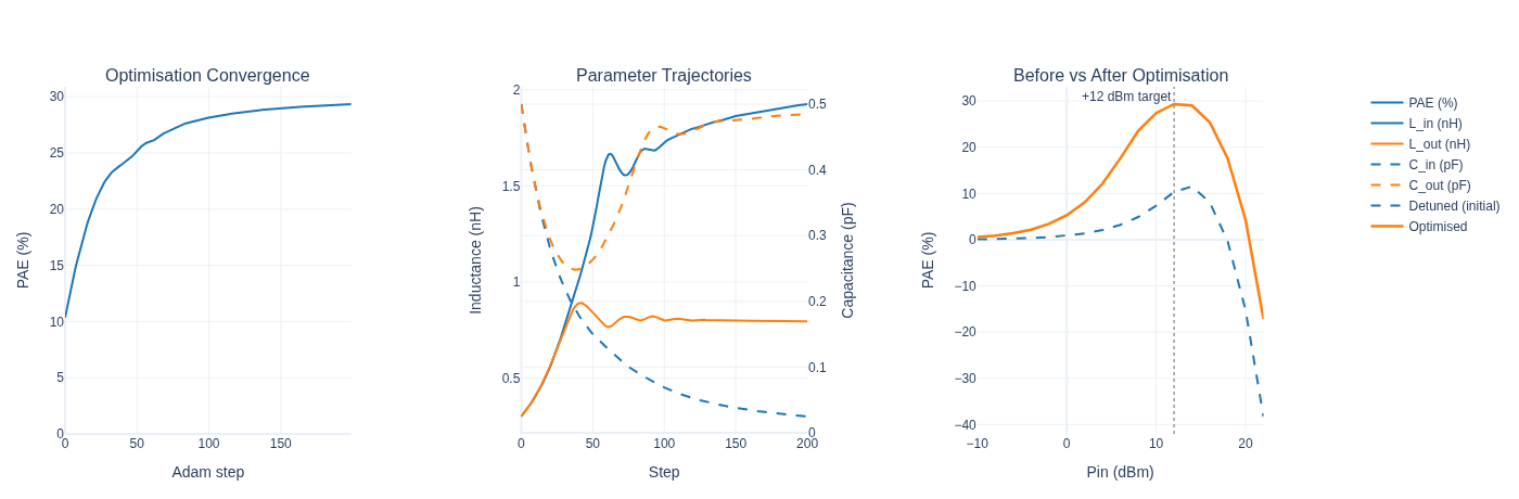
Adam optimisation  (lr = 0.03,  200 steps)
  Step   PAE (%)    L_in (nH)    C_in (pF)    L_out (nH)    C_out (pF)
----------------------------------------------------------------------


     0      10.3        0.309        0.485         0.309         0.485


    50      25.1        1.322        0.148         0.832         0.266


   100      28.1        1.732        0.068         0.800         0.462


   150      29.0        1.865        0.038         0.799         0.475


   199      29.3        1.926        0.025         0.796         0.485

Optimised matching network:
  L_in  = 1.926 nH   (was 0.3 nH)
  C_in  = 0.025 pF   (was 0.5 pF)
  L_out = 0.796 nH   (was 0.3 nH)
  C_out = 0.485 pF   (was 0.5 pF)

Final PAE: 29.3%  (initial: 10.3%)
# ── Build optimised parameter set for before/after comparison ────────────────────────
L_in_f, C_in_f, L_out_f, C_out_f = jnp.exp(log_params)


def run_at_amplitude_opt(V_in):
    _, y_freq_i = _run_pa_hb(
        _pa_params(V_in=V_in, L_in=L_in_f, C_in=C_in_f, L_out=L_out_f, C_out=C_out_f),
        y_flat_init=jnp.tile(y_dc, K),
    )
    _, _, PAE = compute_powers(y_freq_i, V_in, Vdd_val)
    return PAE


run_at_amp_opt_jit = jax.jit(run_at_amplitude_opt)
PAE_opt_list = [float(run_at_amp_opt_jit(jnp.array(V_in))) * 100 for V_in in V_amp_vals]

# ── Plotly figures ────────────────────────────────────────────────────────────────────
param_arr  = np.array(param_history)
steps_arr  = list(np.arange(len(param_arr)))
pae_steps  = list(np.arange(len(pae_history)))

specs = [[{}, {"secondary_y": True}, {}]]
fig = make_subplots(
    rows=1, cols=3,
    subplot_titles=("Optimisation Convergence", "Parameter Trajectories", "Before vs After Optimisation"),
    specs=specs,
)

# Panel 1: PAE convergence
fig.add_trace(
    go.Scatter(x=pae_steps, y=pae_history, mode="lines",
               name="PAE (%)", line=dict(color="#1f77b4", width=2)),
    row=1, col=1,
)

# Panel 2: Parameter trajectories (inductances primary y, capacitances secondary y)
fig.add_trace(
    go.Scatter(x=steps_arr, y=list(param_arr[:, 0] * 1e9), mode="lines",
               name="L_in (nH)", line=dict(color="#1f77b4", width=2)),
    row=1, col=2,
)
fig.add_trace(
    go.Scatter(x=steps_arr, y=list(param_arr[:, 2] * 1e9), mode="lines",
               name="L_out (nH)", line=dict(color="#ff7f0e", width=2)),
    row=1, col=2,
)
fig.add_trace(
    go.Scatter(x=steps_arr, y=list(param_arr[:, 1] * 1e12), mode="lines",
               name="C_in (pF)", line=dict(color="#1f77b4", width=2, dash="dash")),
    row=1, col=2, secondary_y=True,
)
fig.add_trace(
    go.Scatter(x=steps_arr, y=list(param_arr[:, 3] * 1e12), mode="lines",
               name="C_out (pF)", line=dict(color="#ff7f0e", width=2, dash="dash")),
    row=1, col=2, secondary_y=True,
)

# Panel 3: Before / after PAE sweep
fig.add_trace(
    go.Scatter(x=list(Pin_dBm_vals), y=PAE_list, mode="lines",
               name="Detuned (initial)", line=dict(color="#1f77b4", width=2, dash="dash")),
    row=1, col=3,
)
fig.add_trace(
    go.Scatter(x=list(Pin_dBm_vals), y=PAE_opt_list, mode="lines",
               name="Optimised", line=dict(color="#ff7f0e", width=2.5)),
    row=1, col=3,
)
fig.add_vline(x=12, line=dict(color="grey", width=1.2, dash="dot"),
              annotation_text="+12 dBm target", annotation_position="top left",
              row=1, col=3)

# Axis labels
fig.update_xaxes(title_text="Adam step", row=1, col=1)
fig.update_yaxes(title_text="PAE (%)", rangemode="tozero", row=1, col=1)
fig.update_xaxes(title_text="Step", row=1, col=2)
fig.update_yaxes(title_text="Inductance (nH)", row=1, col=2, secondary_y=False)
fig.update_yaxes(title_text="Capacitance (pF)", row=1, col=2, secondary_y=True)
fig.update_xaxes(title_text="Pin (dBm)", row=1, col=3)
fig.update_yaxes(title_text="PAE (%)", rangemode="tozero", row=1, col=3)

fig.update_layout(margin=dict(t=80, b=60, l=60, r=60), height=460, width=1400)
fig.show()
# ── Run HB at optimised matching, target drive level ───────────────────────────────────
y_time_opt, y_freq_opt = _run_pa_hb(
    _pa_params(V_in=V_target, L_in=L_in_f, C_in=C_in_f, L_out=L_out_f, C_out=C_out_f),
    y_flat_init=jnp.tile(y_dc, K),
)

T    = 1.0 / F0                                       # period [s]
t_ps = np.linspace(0, T * 1e12, K, endpoint=False)   # time axis [ps]

v_gate  = np.real(np.array(circuit.port(y_time_opt, "gate")))
v_drain = np.real(np.array(circuit.port(y_time_opt, "drain")))
i_drain = np.real(np.array(y_time_opt[:, choke_iL_idx]))

Pout_opt, Gain_opt, PAE_opt_val = compute_powers(y_freq_opt, V_target, Vdd_val)

harmonics    = np.arange(N_HARM + 1)
scale        = np.where(harmonics == 0, 1.0, 2.0)
spectrum     = scale * np.abs(np.array(circuit.port(y_freq_opt, "drain")[:N_HARM + 1]))
tick_labels  = ["DC" if k == 0 else f"{k}f₀" for k in harmonics]
i_dc_bias    = float(jnp.real(y_freq_opt[0, choke_iL_idx])) * 1e3

fig = make_subplots(
    rows=1, cols=3,
    subplot_titles=("Gate and Drain Waveforms (1 period)", "Drain Current Waveform", "Drain Voltage Spectrum"),
)

# Panel 1: Gate and drain voltages
fig.add_trace(
    go.Scatter(x=list(t_ps), y=list(v_gate), mode="lines+markers",
               name="Gate (V)", marker=dict(size=5), line=dict(color="#1f77b4")),
    row=1, col=1,
)
fig.add_trace(
    go.Scatter(x=list(t_ps), y=list(v_drain), mode="lines+markers",
               name="Drain (V)", marker=dict(size=5), line=dict(color="#ff7f0e")),
    row=1, col=1,
)
fig.add_hline(y=Vdd_val, line=dict(color="grey", width=1, dash="dash"),
              annotation_text=f"Vdd = {Vdd_val} V", annotation_position="bottom right",
              row=1, col=1)

# Panel 2: Drain current
fig.add_trace(
    go.Scatter(x=list(t_ps), y=list(i_drain * 1e3), mode="lines+markers",
               name="Drain current (mA)", marker=dict(size=5), line=dict(color="#2ca02c")),
    row=1, col=2,
)
fig.add_hline(y=i_dc_bias, line=dict(color="grey", width=1.2, dash="dash"),
              annotation_text=f"DC bias = {i_dc_bias:.1f} mA", annotation_position="bottom right",
              row=1, col=2)

# Panel 3: Harmonic spectrum bar chart
fig.add_trace(
    go.Bar(x=list(harmonics), y=list(spectrum * 1e3),
           name="Spectrum (mV)", marker=dict(color="#1f77b4", opacity=0.85,
           line=dict(color="white", width=1))),
    row=1, col=3,
)
fig.update_xaxes(
    tickmode="array", tickvals=list(harmonics), ticktext=tick_labels,
    title_text="Harmonic", row=1, col=3,
)

fig.update_xaxes(title_text="Time (ps)", row=1, col=1)
fig.update_yaxes(title_text="Voltage (V)", row=1, col=1)
fig.update_xaxes(title_text="Time (ps)", row=1, col=2)
fig.update_yaxes(title_text="Drain current (mA)", row=1, col=2)
fig.update_yaxes(title_text="Amplitude (mV)", row=1, col=3)

fig.update_layout(margin=dict(t=80, b=60, l=60, r=60), height=440, width=1400)
fig.show()

print("\nOptimised PA — final performance at +12 dBm input:")
print(f"  Pout = {float(Pout_opt):.1f} dBm")
print(f"  Gain = {float(Gain_opt):.1f} dB")
print(f"  PAE  = {float(PAE_opt_val)*100:.1f}%")
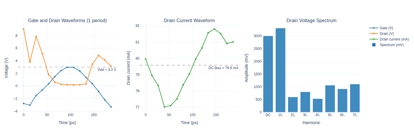
Optimised PA — final performance at +12 dBm input:
  Pout = 19.3 dBm
  Gain = 7.3 dB
  PAE  = 29.3%


Pre-computing 41 PAE sweeps x 17 Pin points...


  [  1/41] step   0 — PAE@+12dBm = 10.3%


  [  6/41] step  25 — PAE@+12dBm = 21.8%


  [ 11/41] step  50 — PAE@+12dBm = 25.1%


  [ 16/41] step  75 — PAE@+12dBm = 27.1%


  [ 21/41] step 100 — PAE@+12dBm = 28.1%


  [ 26/41] step 125 — PAE@+12dBm = 28.7%


  [ 31/41] step 150 — PAE@+12dBm = 29.0%


  [ 36/41] step 175 — PAE@+12dBm = 29.2%


  [ 41/41] step 199 — PAE@+12dBm = 29.3%
Done.


Saved → examples/inverse_design/pa_optimisation.gif
Frames: 41   Duration: 4.1s at 10 fps
Summary¤
Matching Network — Initial vs Optimised¤
| Component | Initial | Role |
|---|---|---|
L_in | 0.3 nH | Input L-match shunt arm |
C_in | 0.5 pF | Input L-match series arm |
L_out | 0.3 nH | Output L-match shunt arm |
C_out | 0.5 pF | Output L-match series arm |
What made this possible¤
| Traditional EDA | Circulax |
|---|---|
| HB solve → hand-tune → re-solve | HB solve → jax.grad → Adam step |
| Gradient-free search (genetic, random) | Exact analytic gradients via implicit differentiation |
| Hundreds of HB evaluations to converge | ~1 adjoint solve per gradient (one extra LU factorisation) |
| Fixed S-parameter models | Fully differentiable device physics (HEMT, diodes, varactors) |
Extending this framework¤
The same gradient infrastructure applies directly to:
- Load-pull contours — sweep complex Γ_L and compute
∂PAE/∂Γ_Lanalytically. - Multi-tone IMD / ACPR — add intermodulation terms to the HB system; differentiate w.r.t. device parameters to minimise distortion.
- Phase noise — perturb the HB fixed point; the linear noise response is the adjoint of the same Jacobian already computed during optimisation.
- Co-design — jointly optimise device epitaxial parameters (β, Vp) and circuit matching, treating the entire design stack as one differentiable programme.