Fitting PSP103 Process Parameters to I-V Measurements¤
Compact-model calibration traditionally requires sweeping a large parameter grid and comparing against measured data — a process that scales poorly with parameter count. Conventional SPICE simulators provide no gradient information, so optimisers must resort to finite-difference (FD) over the entire simulation: \(N_{params}\) extra DC solves per bias point.
circulax solves this with a discrete adjoint method. Because the circuit topology is assembled in JAX, the Jacobian and its transpose solve come for free from the existing Newton factorisation. Only the per-parameter device physics — the part that lives inside the OSDI binary — is evaluated via FD, and each FD probe is a single lightweight osdi_residual_eval call (not a full circuit solve). The result: one adjoint linear solve + \(N_{params}\) cheap OSDI evaluations replaces \(N_{params}\) full DC solves.
| Conventional SPICE | circulax DC adjoint | |
|---|---|---|
| Gradient method | FD over full DC solve | Adjoint solve + FD through OSDI residual only |
| Cost per bias point | \(N_p + 1\) DC solves | 1 DC solve + 1 adjoint solve + \(N_p\) OSDI evals |
| Scales with | Circuit size × \(N_p\) | Circuit size + \(N_p\) (decoupled) |
| Requires model source? | Often yes (for internal FD) | No — works with compiled .osdi binaries |
This example uses the PSP103 MOSFET model compiled to an .osdi binary by openvaf-reloaded and loaded via the bosdi FFI layer. circulax currently requires OSDI API version 0.4.
What you will learn¤
- Loading a Verilog-A compact model via
osdi_component - Building a single-MOSFET I-V test bench with the
CircuitAPI - Computing DC parameter gradients with
dc_parameter_sensitivity - Log-space optimisation for multi-scale parameters
- Recovering process parameters from noisy I-V measurements
import json
import time
from pathlib import Path

import equinox as eqx
import jax
import jax.numpy as jnp
import matplotlib.pyplot as plt
import numpy as np
import optax

from circulax import compile_circuit, osdi_component, update_params_dict
from circulax.components.electronic import VoltageSource
from circulax.solvers import dc_parameter_sensitivity
from circulax.solvers.sensitivity import _resolve_param_cols

jax.config.update("jax_enable_x64", True)
1. Load the PSP103 OSDI Model¤
osdi_component loads a compiled Verilog-A .osdi binary and creates a model descriptor that compile_circuit can use directly. The 783-parameter model card is loaded from a reference JSON file.
DATA_DIR = Path("tests/data/va/psp103v4")

for candidate in [DATA_DIR, Path.cwd().parents[1] / DATA_DIR]:
    if (candidate / "psp103.osdi").exists():
        DATA_DIR = candidate
        break

PSP103_OSDI = DATA_DIR / "psp103.osdi"

with open(DATA_DIR / "psp103_defaults.json") as f:
    nmos_defaults = json.load(f)

psp103n = osdi_component(
    osdi_path=str(PSP103_OSDI),
    ports=("D", "G", "S", "B"),
    default_params=nmos_defaults,
)


def geom_settings(w, length, ld=0.5e-6, ls=0.5e-6):
    return {
        "W": w, "L": length,
        "AD": w * ld, "AS": w * ls,
        "PD": 2.0 * (w + ld), "PS": 2.0 * (w + ls),
    }


NMOS_GEOM = geom_settings(10e-6, 1e-6)

PARAM_NAMES = ["VFBO", "NSUBO", "TOXO", "UO", "MUEO", "THEMUO"]

print(f"Loaded PSP103 from {PSP103_OSDI}")
print(f"  Pins:   {psp103n.ports}")
print(f"  Params: {len(psp103n.param_names)}")
print(f"  Fitting: {PARAM_NAMES}")
Loaded PSP103 from tests/data/va/psp103v4/psp103.osdi
  Pins:   ('D', 'G', 'S', 'B')
  Params: 783
  Fitting: ['VFBO', 'NSUBO', 'TOXO', 'UO', 'MUEO', 'THEMUO']
2. Build the Test Circuit¤
A single NMOS transistor with gate and drain voltage sources. Source and bulk are tied to ground.
compile_circuit handles netlist compilation and solver setup in one call, returning a Circuit object. We extract the drain-current index from the port map — it corresponds to the internal current variable of the Vds voltage source.
net_dict = {
    "instances": {
        "M1":  {"component": "nmos", "settings": {**NMOS_GEOM}},
        "Vgs": {"component": "vsrc", "settings": {"V": 0.0}},
        "Vds": {"component": "vsrc", "settings": {"V": 1.0}},
    },
    "connections": {
        "Vgs,p1": "gate,p1",  "Vgs,p2": "GND,p1",
        "Vds,p1": "drain,p1", "Vds,p2": "GND,p1",
        "M1,G": "gate,p1",
        "M1,D": "drain,p1",
        "M1,S": "GND,p1",
        "M1,B": "GND,p1",
    },
    "ports": {},
}
models = {"nmos": psp103n, "vsrc": VoltageSource}

circuit = compile_circuit(net_dict, models, is_complex=False)

id_idx = circuit.port_map["Vds,i_src"]
print(f"System size: {circuit.sys_size}")
print(f"Drain current index (i_src of Vds): {id_idx}")

param_cols = _resolve_param_cols(
    circuit.groups["nmos"], PARAM_NAMES, model_descriptor=psp103n,
)
param_cols_map = dict(zip(PARAM_NAMES, param_cols))

nominal_params = np.array(jax.device_get(circuit.groups["nmos"].params))
nominal_vals = {p: float(nominal_params[0, param_cols_map[p]]) for p in PARAM_NAMES}

print("\nNominal parameter values:")
for p in PARAM_NAMES:
    print(f"  {p:8s} = {nominal_vals[p]:12.4e}")
System size: 7
Drain current index (i_src of Vds): 3

Nominal parameter values:
  VFBO     =  -1.1000e+00
  NSUBO    =   3.0000e+23
  TOXO     =   1.5000e-09
  UO       =   3.5000e-02
  MUEO     =   6.0000e-01
  THEMUO   =   2.7500e+00
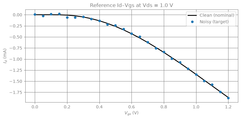
3. Generate Reference I-V Data¤
We sweep \(V_{gs}\) from 0 to 1.2 V at \(V_{ds}\) = 1.0 V using the nominal PSP103 parameters to produce a "ground truth" \(I_d\)–\(V_{gs}\) curve, then add Gaussian noise to simulate measurement uncertainty.
Passing an array-valued parameter to circuit.dc() automatically vmaps the Newton solver over all bias points in a single JIT-compiled call.
VGS_SWEEP = jnp.linspace(0.0, 1.2, 25)

t0 = time.time()
y_batch = circuit.dc(params={"Vgs.V": VGS_SWEEP})
t_sweep = time.time() - t0

id_ref = np.array(jax.device_get(y_batch[:, id_idx]))

rng = np.random.default_rng(42)
noise_sigma = 25e-6
id_ref_noisy = id_ref + rng.normal(0, noise_sigma, size=id_ref.shape)

print(f"DC sweep ({len(VGS_SWEEP)} points, vmapped): {t_sweep:.2f} s")
print(f"Id range: {id_ref.min() * 1e3:.3f} mA to {id_ref.max() * 1e3:.3f} mA")
DC sweep (25 points, vmapped): 0.62 s
Id range: -1.867 mA to -0.000 mA
fig, ax = plt.subplots(figsize=(8, 4))
ax.plot(VGS_SWEEP, id_ref * 1e3, "k-", lw=2, label="Clean (nominal)")
ax.plot(VGS_SWEEP, id_ref_noisy * 1e3, "o", ms=5, color="C0", label="Noisy (target)")
ax.set_xlabel("$V_{gs}$ (V)")
ax.set_ylabel("$I_d$ (mA)")
ax.set_title("Reference Id\u2013Vgs at Vds = 1.0 V")
ax.legend()
plt.tight_layout()
4. DC Adjoint Parameter Fitting¤
Why not just autodiff?¤
For JAX-native components (resistors, capacitors, custom elements), circulax can differentiate through the entire simulation with jax.grad — both w.r.t. voltages and parameters. OSDI models support autodiff w.r.t. voltages (via analytical Jacobians returned by the .osdi binary and a @custom_jvp rule in bosdi), which is how circulax assembles \(J = \partial F / \partial y\) for Newton iteration. However, autodiff w.r.t. model parameters is not available through the OSDI ABI — the compiled binary treats parameters as fixed constants.
Note: bosdi also provides an experimental VA-to-JAX lowering path (
bosdi.va) that compiles Verilog-A source directly into pure JAX, making the model fully differentiable w.r.t. voltages, parameters, and temperature. When that path matures,jax.gradwould replace the adjoint method entirely. This notebook uses the stable OSDI binary path.
The adjoint decomposition¤
dc_parameter_sensitivity bridges this gap by splitting the gradient into two parts:
- Adjoint solve (\(J^\top \lambda = \partial\mathcal{L}/\partial y\)): reuses the KLU factorisation from the DC Newton solver — essentially free.
- Parameter Jacobian (\(\partial F / \partial p_k\)): forward FD through
osdi_residual_evalonly — one cheap FFI call per parameter, not a full circuit solve.
The adjoint method itself is not unique to circulax — any simulator with a transpose linear solve and per-parameter residual evaluation could implement it. What circulax provides is the differentiable ecosystem: the adjoint gradients flow directly into JAX optimisers (optax), compose with arbitrary loss functions via autodiff, and integrate with the broader JAX scientific computing stack (Diffrax, Optimistix, equinox) without glue code.
JIT-compiled multi-start optimisation¤
Because the Newton solver, KLU transpose solve, and OSDI FFI evaluations are all XLA custom calls, the entire optimisation loop can be compiled with jax.jit and iterated with jax.lax.scan. This eliminates Python-loop overhead and enables jax.vmap over multiple random starting points — running \(K\) independent Adam trajectories in parallel to guard against local minima.
Log-space parametrisation¤
We optimise in log-space (\(\theta_k = \log |p_k|\)) so that parameters spanning many orders of magnitude receive comparable gradient magnitudes:
N_OPT = 40
LR = 0.02
K_STARTS = 8

optimizer = optax.adam(LR)
nominal_jax = jnp.array(nominal_params, dtype=jnp.float64)
param_cols_arr = jnp.array(param_cols)
n_fit = len(PARAM_NAMES)
id_ref_noisy_jax = jnp.array(id_ref_noisy)

nmos_base = circuit.groups["nmos"].without_handle()
base_groups = {**circuit.groups, "nmos": nmos_base}

rng2 = np.random.default_rng(0)
all_log_params, all_signs = [], []
for k in range(K_STARTS):
    pert = 1.0 + 0.15 * rng2.choice([-1.0, 1.0], size=n_fit)
    current = nominal_params.copy()
    for j, p in enumerate(PARAM_NAMES):
        current[0, param_cols_map[p]] *= pert[j]
    all_signs.append([np.sign(current[0, param_cols_map[p]]) for p in PARAM_NAMES])
    all_log_params.append([np.log(abs(current[0, param_cols_map[p]])) for p in PARAM_NAMES])

log_params_batch = jnp.array(all_log_params)
signs_batch = jnp.array(all_signs)

print(f"Multi-start setup: {K_STARTS} starts x {N_OPT} Adam steps x {len(VGS_SWEEP)} bias points")
print(f"  = {K_STARTS * N_OPT * len(VGS_SWEEP):,} DC solves + sensitivities (vmapped)")
Multi-start setup: 8 starts x 40 Adam steps x 25 bias points
  = 8,000 DC solves + sensitivities (vmapped)
def run_optimization(log_params_init, signs):
    """Run N_OPT Adam steps from a single starting point (JIT + lax.scan)."""
    sys_size = circuit.sys_size

    def opt_step(carry, _):
        log_params, opt_state = carry
        p = nominal_jax.at[0, param_cols_arr].set(signs * jnp.exp(log_params))
        nmos = eqx.tree_at(lambda g: g.params, nmos_base, p)
        groups = {**base_groups, "nmos": nmos}

        total_loss = jnp.float64(0.0)
        log_grad = jnp.zeros(n_fit, dtype=jnp.float64)
        y_prev = jnp.zeros(sys_size, dtype=jnp.float64)

        for i in range(len(VGS_SWEEP)):
            g = update_params_dict(groups, "vsrc", "Vgs", "V", VGS_SWEEP[i])
            y_star = circuit.solver.solve_dc(g, y_prev)
            y_prev = y_star

            id_target = id_ref_noisy_jax[i]
            total_loss = total_loss + (y_star[id_idx] - id_target) ** 2

            grads = dc_parameter_sensitivity(
                g, circuit.solver, y_star,
                lambda y, _t=id_target: (y[id_idx] - _t) ** 2,
                osdi_group_key="nmos", param_names=PARAM_NAMES,
                model_descriptor=psp103n,
            )
            p_vals = jnp.array([p[0, param_cols_map[pn]] for pn in PARAM_NAMES])
            raw_g = jnp.array([grads[pn][0] for pn in PARAM_NAMES])
            log_grad = log_grad + raw_g * p_vals

        updates, new_opt_state = optimizer.update(log_grad, opt_state)
        new_lp = optax.apply_updates(log_params, updates)
        return (new_lp, new_opt_state), total_loss

    init = (log_params_init, optimizer.init(log_params_init))
    (final_lp, _), losses = jax.lax.scan(opt_step, init, jnp.arange(N_OPT))
    return final_lp, losses


multi_optimize = jax.jit(jax.vmap(run_optimization))

t_opt_start = time.time()
print(f"Compiling and running {K_STARTS} parallel optimisations...")
all_final_lp, all_losses = multi_optimize(log_params_batch, signs_batch)
jax.block_until_ready(all_final_lp)
t_opt = time.time() - t_opt_start

best_idx = int(jnp.argmin(all_losses[:, -1]))
print(f"Total time: {t_opt:.1f} s ({K_STARTS} starts, {N_OPT} steps each)")
print("\nFinal losses per start:")
for k in range(K_STARTS):
    marker = " <-- best" if k == best_idx else ""
    print(f"  Start {k}: {float(all_losses[k, -1]):.4e}{marker}")
Compiling and running 8 parallel optimisations...


Total time: 11.5 s (8 starts, 40 steps each)

Final losses per start:
  Start 0: 1.1542e-08 <-- best
  Start 1: 1.6524e-08
  Start 2: 1.1700e-08
  Start 3: 7.6226e-08
  Start 4: 7.1719e-08
  Start 5: 1.4308e-08
  Start 6: 1.2273e-08
  Start 7: 1.6524e-08
best_lp = all_final_lp[best_idx]
best_signs = signs_batch[best_idx]
best_params = nominal_params.copy()
for j, p in enumerate(PARAM_NAMES):
best_params[0, param_cols_map[p]] = float(best_signs[j] * jnp.exp(best_lp[j]))
nmos_final = circuit.groups["nmos"].with_params(
jnp.array(best_params, dtype=jnp.float64),
)
circuit_final = circuit.with_groups({**circuit.groups, "nmos": nmos_final})
y_final = circuit_final.dc(params={"Vgs.V": VGS_SWEEP})
id_final = np.array(jax.device_get(y_final[:, id_idx]))
init_lp = log_params_batch[best_idx]
init_params = nominal_params.copy()
for j, p in enumerate(PARAM_NAMES):
init_params[0, param_cols_map[p]] = float(best_signs[j] * jnp.exp(init_lp[j]))
nmos_init = circuit.groups["nmos"].with_params(
jnp.array(init_params, dtype=jnp.float64),
)
circuit_init = circuit.with_groups({**circuit.groups, "nmos": nmos_init})
y_init = circuit_init.dc(params={"Vgs.V": VGS_SWEEP})
id_init = np.array(jax.device_get(y_init[:, id_idx]))
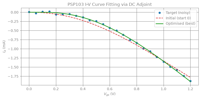
fig, ax = plt.subplots(figsize=(8, 4))
ax.plot(VGS_SWEEP, id_ref_noisy * 1e3, "o", ms=5, color="C0", label="Target (noisy)")
ax.plot(VGS_SWEEP, id_init * 1e3, "--", color="C3", lw=1.5, label=f"Initial (start {best_idx})")
ax.plot(VGS_SWEEP, id_final * 1e3, "-", color="C2", lw=2, label="Optimised (best)")
ax.set_xlabel("$V_{gs}$ (V)")
ax.set_ylabel("$I_d$ (mA)")
ax.set_title("PSP103 I-V Curve Fitting via DC Adjoint")
ax.legend()
plt.tight_layout()
log_nominal = np.log(np.abs(np.array([nominal_vals[p] for p in PARAM_NAMES])))
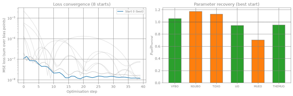
fig, (ax1, ax2) = plt.subplots(1, 2, figsize=(12, 4))
for k in range(K_STARTS):
alpha = 1.0 if k == best_idx else 0.2
color = "C0" if k == best_idx else "grey"
label = f"Start {k} (best)" if k == best_idx else ("Others" if k == 0 else None)
ax1.semilogy(np.array(all_losses[k]), color=color, alpha=alpha, lw=1.5, label=label)
ax1.set_xlabel("Optimisation step")
ax1.set_ylabel("MSE loss (sum over bias points)")
ax1.set_title(f"Loss convergence ({K_STARTS} starts)")
ax1.legend(fontsize=8)
ratios = []
for j, p in enumerate(PARAM_NAMES):
opt_val = best_params[0, param_cols_map[p]]
ratios.append(opt_val / nominal_vals[p])
x = np.arange(n_fit)
colors = ["C2" if abs(r - 1) < 0.1 else "C1" for r in ratios]
ax2.bar(x, ratios, color=colors, edgecolor="grey", width=0.6)
ax2.axhline(1.0, color="k", ls=":", lw=0.8)
ax2.set_xticks(x)
ax2.set_xticklabels(PARAM_NAMES, fontsize=8)
ax2.set_ylabel("$p_{opt} / p_{nominal}$")
ax2.set_title("Parameter recovery (best start)")
plt.tight_layout()
print(f"Parameter recovery (best of {K_STARTS} starts):")
fmt = "  {:10s}  {:>12s}  {:>12s}  {:>8s}"
print(fmt.format("Parameter", "Nominal", "Optimised", "Error"))
print("  " + "-" * 48)
for j, p in enumerate(PARAM_NAMES):
    nom = nominal_vals[p]
    opt_val = best_params[0, param_cols_map[p]]
    err = abs(opt_val - nom) / abs(nom) * 100
    print(f"  {p:10s}  {nom:12.4e}  {opt_val:12.4e}  {err:7.2f}%")
Parameter recovery (best of 8 starts):
  Parameter        Nominal     Optimised     Error
  ------------------------------------------------
  VFBO         -1.1000e+00   -1.1606e+00     5.51%
  NSUBO         3.0000e+23    3.5214e+23    17.38%
  TOXO          1.5000e-09    1.6920e-09    12.80%
  UO            3.5000e-02    3.2959e-02     5.83%
  MUEO          6.0000e-01    4.2183e-01    29.69%
  THEMUO        2.7500e+00    2.6190e+00     4.76%
Summary¤
| Stage | What happened |
|---|---|
| OSDI model loaded | PSP103 .osdi binary with 783 parameters via osdi_component |
| Test circuit | Single NMOS with Vgs/Vds sources — compile_circuit handles compilation + solver setup |
| Reference data | 25-point Id-Vgs sweep with Gaussian noise |
| Gradient method | dc_parameter_sensitivity — adjoint (topology via JAX) + FD (physics via OSDI) |
| Optimisation | jax.vmap over 8 starting points, each running 40 Adam steps via lax.scan |
The entire optimisation loop — Newton solve, adjoint solve, OSDI residual evaluations — compiles to a single XLA program via jax.jit. jax.vmap runs multiple random starting points in parallel with zero additional compilation cost, guarding against local minima.
Going further¤
- More parameters: add geometry (W, L) or doping profile parameters
- Multi-output: fit Id-Vgs and Id-Vds families simultaneously
- Transient fitting: use
transient_parameter_sensitivityfor time-domain data - Full autodiff: bosdi's experimental VA-to-JAX lowering compiles Verilog-A source into pure JAX — when mature,
jax.gradwill replace the adjoint method entirely