AC Sweep

AC Small-Signal Analysis (S-parameters)¤

This notebook demonstrates setup_ac_sweep on two circuits:

Parallel RC — single port — a minimal benchmark. We compare \(S_{11}(f)\) against the analytical admittance formula.
Series-R shunt-C lowpass — two ports — a classic LC prototype filter. We recover all four S-parameters and verify passivity.
Skin-effect resistor (fdomain component) — a frequency-dependent component whose impedance \(Z(f) = R_0 + a\sqrt{f}\) cannot be expressed as a time-domain DAE; @fdomain_component handles it natively.

AC analysis linearises the circuit DAE at the DC operating point and sweeps a range of frequencies:

\[Y(j\omega) = G + j\omega C, \qquad G = \partial F/\partial y\big|_{y_\text{dc}}, \quad C = \partial Q/\partial y\big|_{y_\text{dc}}\]

With \(N\) port excitations as columns of the RHS, a single jnp.linalg.solve per frequency yields the full \(N\times N\) S-matrix at once.

import jax
import jax.numpy as jnp
import matplotlib.pyplot as plt
import numpy as np
import schemdraw
import schemdraw.elements as elm

from circulax import compile_circuit, fdomain_component, setup_ac_sweep
from circulax.components.electronic import Capacitor, Resistor

jax.config.update("jax_enable_x64", True)

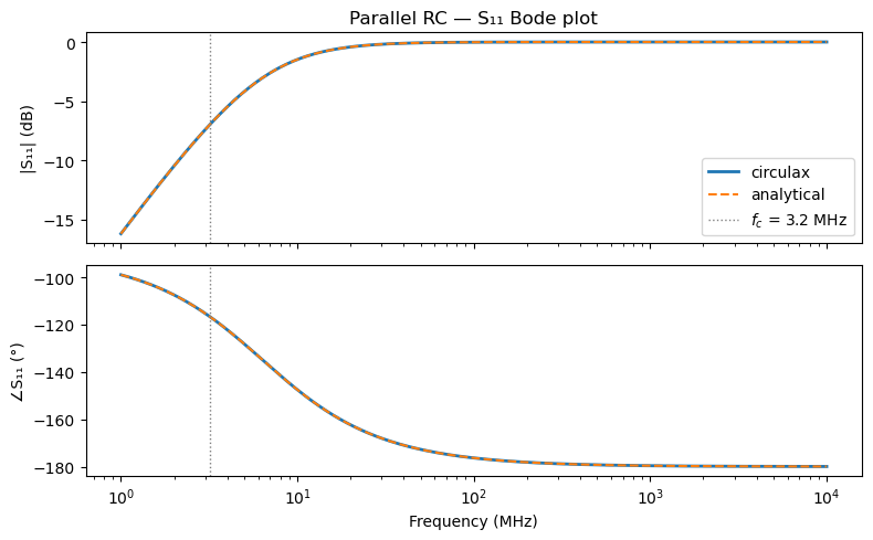
Part 1: Parallel RC — Single Port¤

A resistor \(R\) and capacitor \(C\) both shunt from the port node to ground. The circuit admittance is \(Y_\text{circuit} = 1/R + j\omega C\), so the analytical \(S_{11}\) is:

\[Y_\text{total} = \frac{1}{Z_0} + \frac{1}{R} + j\omega C, \qquad S_{11} = \frac{2/Z_0}{Y_\text{total}} - 1\]

At DC (\(\omega\to 0\)) the capacitor is an open circuit. For \(R = Z_0 = 50\,\Omega\) we get the classic matched-load result \(S_{11}(0) = 0\). At high frequencies \(C\) short-circuits \(R\) so \(S_{11} \to -1\).

R = 50.0  # Ω  (shunt resistor = Z0 → matched at DC)
C = 1e-9  # F  (1 nF shunt capacitor)
Z0 = 50.0  # Ω  (reference impedance)

f_c = 1.0 / (2 * np.pi * R * C)  # RC corner frequency
print(f"RC corner frequency: {f_c / 1e6:.3f} MHz")

with plt.style.context(["default", {"axes.grid": True, "figure.facecolor": "white"}]), schemdraw.Drawing() as d:
    d.config(fontsize=12, unit=3.0)
    d.add(elm.Dot(open=True).label("Port 1", loc="left"))
    d.add(elm.Line().right(d.unit * 0.8))
    top = d.here
    d.add(elm.Dot())
    d.add(elm.Resistor().down().label(f"$R$\n{R:.0f} Ω", loc="right"))
    d.add(elm.Ground())
    d.add(elm.Line().right(d.unit).at(top))
    d.add(elm.Capacitor().down().label(f"$C$\n{C * 1e9:.0f} nF", loc="right"))
    d.add(elm.Ground())

RC corner frequency: 3.183 MHz

models = {"resistor": Resistor, "capacitor": Capacitor, "ground": lambda: 0}

net_rc = {
    "instances": {
        "GND": {"component": "ground"},
        "R1": {"component": "resistor", "settings": {"R": R}},
        "C1": {"component": "capacitor", "settings": {"C": C}},
    },
    "connections": {
        "R1,p1": "C1,p1",  # shared port node
        "R1,p2": "GND,p1",
        "C1,p2": "GND,p1",
    },
}

circuit = compile_circuit(net_rc, models)
y_dc = circuit()

port_nodes = [circuit.port_map["R1,p1"]]
run_ac = setup_ac_sweep(circuit.groups, circuit.sys_size, port_nodes, z0=Z0)

freqs = jnp.logspace(6, 10, 300)  # 1 MHz → 10 GHz
S = jax.jit(run_ac)(y_dc, freqs)
S11 = S[:, 0, 0]
print(f"S shape: {S.shape}  (N_freqs, N_ports, N_ports)")

S shape: (300, 1, 1)  (N_freqs, N_ports, N_ports)

# Analytical reference
omega = 2 * jnp.pi * freqs
Y_total = 1.0 / Z0 + 1.0 / R + 1j * omega * C
S11_ref = (2.0 / Z0) / Y_total - 1.0

max_err = float(jnp.max(jnp.abs(S11 - S11_ref)))
print(f"Max |ΔS11| = {max_err:.2e}")

fig, (ax1, ax2) = plt.subplots(2, 1, figsize=(8, 5), sharex=True)

ax1.semilogx(freqs / 1e6, 20 * np.log10(np.abs(S11)), "C0", lw=2, label="circulax")
ax1.semilogx(freqs / 1e6, 20 * np.log10(np.abs(S11_ref)), "C1--", lw=1.5, label="analytical")
ax1.axvline(f_c / 1e6, color="gray", ls=":", lw=1, label=f"$f_c$ = {f_c / 1e6:.1f} MHz")
ax1.set_ylabel("|S₁₁| (dB)")
ax1.set_title("Parallel RC — S₁₁ Bode plot")
ax1.legend()

ax2.semilogx(freqs / 1e6, np.degrees(np.angle(S11)), "C0", lw=2)
ax2.semilogx(freqs / 1e6, np.degrees(np.angle(S11_ref)), "C1--", lw=1.5)
ax2.axvline(f_c / 1e6, color="gray", ls=":", lw=1)
ax2.set_ylabel("∠S₁₁ (°)")
ax2.set_xlabel("Frequency (MHz)")

plt.tight_layout()
plt.show()

Max |ΔS11| = 4.00e-11

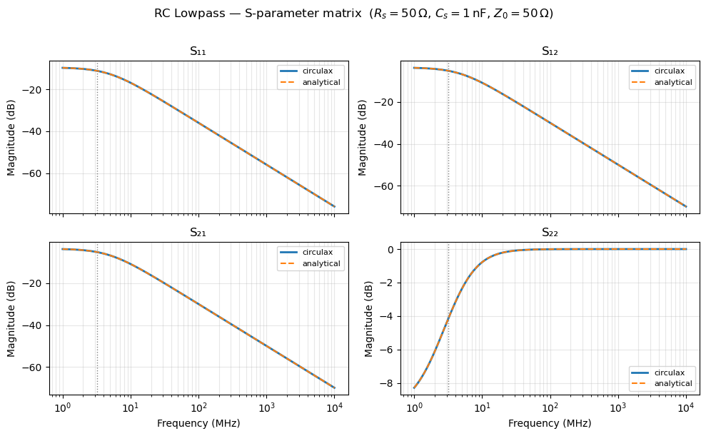
Part 2: RC Lowpass Filter — Two Ports¤

A series resistor \(R_s\) followed by a shunt capacitor \(C_s\) forms a first-order lowpass prototype. With \(Z_0\) terminations at both ports the 3 dB cutoff is approximately:

\[f_{\text{3dB}} \approx \frac{1}{2\pi R_s C_s}\]

At low frequencies energy passes through (\(|S_{21}| \approx 0\,\text{dB}\)); at high frequencies the capacitor short-circuits the output (\(|S_{21}| \to -\infty\,\text{dB}\)).

Passivity requires \(|S_{11}|^2 + |S_{21}|^2 \leq 1\) at all frequencies (for a lossless 2-port with a single incident wave).

R_s = 50.0  # Ω  series
C_s = 1e-9  # F  shunt

f_3dB = 1.0 / (2 * np.pi * R_s * C_s)
print(f"Approximate 3 dB frequency: {f_3dB / 1e6:.3f} MHz")

with plt.style.context(["default", {"axes.grid": True, "figure.facecolor": "white"}]), schemdraw.Drawing() as d:
    d.config(fontsize=12, unit=3.0)
    d.add(elm.Dot(open=True).label("Port 1", loc="left"))
    rs = d.add(elm.Resistor().right().label(f"$R_s$\n{R_s:.0f} Ω"))
    jct = d.here
    d.add(elm.Dot())
    d.add(elm.Dot(open=True).label("Port 2", loc="right"))
    d.add(elm.Capacitor().down().at(jct).label(f"$C_s$\n{C_s * 1e9:.0f} nF", loc="right"))
    d.add(elm.Ground())

Approximate 3 dB frequency: 3.183 MHz

# Port 1 is R1,p1 — a large shunt resistor (1 TΩ) registers it as a circuit node
# with negligible effect on the result (contributes 1e-12 S vs 1/Z0 = 0.02 S).
net_lp = {
    "instances": {
        "GND": {"component": "ground"},
        "Rprobe": {"component": "resistor", "settings": {"R": 1e15}},  # 1 TΩ port probe
        "R1": {"component": "resistor", "settings": {"R": R_s}},
        "C1": {"component": "capacitor", "settings": {"C": C_s}},
    },
    "connections": {
        "Rprobe,p1": "R1,p1",  # port 1 node
        "Rprobe,p2": "GND,p1",
        "R1,p2": "C1,p1",  # junction = port 2 node
        "C1,p2": "GND,p1",
    },
}

circuit_lp = compile_circuit(net_lp, models)
y_dc_lp = circuit_lp()

port_nodes_lp = [circuit_lp.port_map["R1,p1"], circuit_lp.port_map["R1,p2"]]
run_ac_lp = setup_ac_sweep(circuit_lp.groups, circuit_lp.sys_size, port_nodes_lp, z0=Z0)

S_lp = jax.jit(run_ac_lp)(y_dc_lp, freqs)
print(f"S shape: {S_lp.shape}  (N_freqs, 2, 2)")

S shape: (300, 2, 2)  (N_freqs, 2, 2)

# Analytical 2×2 reference: solve the nodal system at each frequency
def _s_analytical_lp(f, R=R_s, C=C_s, Z0=Z0):
    omega = 2 * jnp.pi * f
    Y = jnp.array(
        [
            [1 / Z0 + 1 / R, -1 / R],
            [-1 / R, 1 / Z0 + 1 / R + 1j * omega * C],
        ],
        dtype=jnp.complex128,
    )
    RHS = (2.0 / Z0) * jnp.eye(2, dtype=jnp.complex128)  # two port excitations
    V = jnp.linalg.solve(Y, RHS)  # (2, 2): columns = solutions per excitation
    return V - jnp.eye(2, dtype=jnp.complex128)


S_ref_lp = jax.vmap(_s_analytical_lp)(freqs)

print("S-parameter max errors vs analytical:")
for i in range(2):
    for j in range(2):
        err = float(jnp.max(jnp.abs(S_lp[:, i, j] - S_ref_lp[:, i, j])))
        print(f"  S{i + 1}{j + 1}: {err:.2e}")

# Passivity: |S11|² + |S21|² ≤ 1 (power conservation, port 1 excitation)
col1_power = jnp.abs(S_lp[:, 0, 0]) ** 2 + jnp.abs(S_lp[:, 1, 0]) ** 2
print(f"\nMax |S11|² + |S21|² = {float(jnp.max(col1_power)):.6f}  (must be ≤ 1)")

fig, axes = plt.subplots(2, 2, figsize=(10, 6), sharex=True)

params = [(0, 0, "S₁₁"), (0, 1, "S₁₂"), (1, 0, "S₂₁"), (1, 1, "S₂₂")]
for i, j, label in params:
    ax = axes[i][j]
    ax.semilogx(freqs / 1e6, 20 * np.log10(np.abs(S_lp[:, i, j])), "C0", lw=2, label="circulax")
    ax.semilogx(freqs / 1e6, 20 * np.log10(np.abs(S_ref_lp[:, i, j])), "C1--", lw=1.5, label="analytical")
    ax.axvline(f_3dB / 1e6, color="gray", ls=":", lw=1)
    ax.set_title(label)
    ax.set_ylabel("Magnitude (dB)")
    ax.legend(fontsize=8)
    ax.grid(True, which="both", alpha=0.3)

for ax in axes[1]:
    ax.set_xlabel("Frequency (MHz)")

plt.suptitle(
    f"RC Lowpass — S-parameter matrix  ($R_s = {R_s:.0f}\\,\\Omega$, $C_s = {C_s * 1e9:.0f}\\,\\text{{nF}}$, $Z_0 = {Z0:.0f}\\,\\Omega$)",
    y=1.01,
)
plt.tight_layout()
plt.show()

S-parameter max errors vs analytical:
  S11: 9.99e-12
  S12: 2.00e-11
  S21: 2.00e-11
  S22: 4.00e-11

Max |S11|² + |S21|² = 0.532210  (must be ≤ 1)

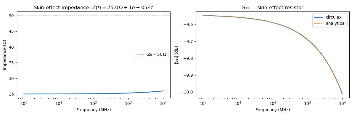
Part 3: Skin-Effect Resistor (`@fdomain_component`)¤

The skin effect causes the resistance of a conductor to increase with frequency:

\[Z(f) = R_0 + a\sqrt{f}\]

where \(R_0\) is the DC resistance and \(a\) is a geometry-dependent coefficient. This impedance has no finite-order rational approximation, so it cannot be expressed as a finite-dimensional time-domain DAE.

Using @fdomain_component, we define the admittance matrix \(Y(f)\) directly. The AC sweep evaluates it at each frequency point inside the jax.vmap loop.

@fdomain_component(ports=("p1", "p2"))
def SkinResistor(f: float, R0: float = 25.0, a: float = 1e-5):
    """Skin-effect resistor: Z(f) = R0 + a·√f  →  Y(f) = 1/Z(f)."""
    Z = R0 + a * jnp.sqrt(jnp.abs(f) + 1e-30)  # 1e-30 regularises f=0
    Y = 1.0 / Z
    return jnp.array([[Y, -Y], [-Y, Y]], dtype=jnp.complex128)


R0, a = 25.0, 1e-5  # Ω,  Ω/√Hz

models_skin = {"skin_r": SkinResistor, "resistor": Resistor, "ground": lambda: 0}

net_skin = {
    "instances": {
        "GND": {"component": "ground"},
        "SR1": {"component": "skin_r", "settings": {"R0": R0, "a": a}},
        "Rbig": {"component": "resistor", "settings": {"R": 1e15}},  # 1 TΩ port probe
    },
    "connections": {
        "SR1,p1": "Rbig,p1",  # port node
        "SR1,p2": "GND,p1",
        "Rbig,p2": "GND,p1",
    },
}

circuit_sk = compile_circuit(net_skin, models_skin)
y_dc_sk = circuit_sk()

run_ac_sk = setup_ac_sweep(circuit_sk.groups, circuit_sk.sys_size, [circuit_sk.port_map["SR1,p1"]], z0=Z0)
S_sk = jax.jit(run_ac_sk)(y_dc_sk, freqs)
S11_sk = S_sk[:, 0, 0]

# Analytical: Z(f) is real so |Γ| = |Z - Z0| / |Z + Z0|
Z_skin = R0 + a * jnp.sqrt(jnp.abs(freqs) + 1e-30)
Y_total_sk = 1.0 / Z0 + 1.0 / Z_skin
S11_sk_ref = (2.0 / Z0) / Y_total_sk - 1.0

max_err_sk = float(jnp.max(jnp.abs(S11_sk - S11_sk_ref)))
print(f"Max |ΔS11| (skin effect) = {max_err_sk:.2e}")

# Show impedance and S11 side by side
fig, (ax1, ax2) = plt.subplots(1, 2, figsize=(12, 4))

ax1.semilogx(freqs / 1e6, np.array(Z_skin), "C0", lw=2)
ax1.set_xlabel("Frequency (MHz)")
ax1.set_ylabel("Impedance (Ω)")
ax1.set_title(f"Skin-effect impedance: $Z(f) = {R0}\\,\\Omega + {a:.0e}\\sqrt{{f}}$")
ax1.axhline(Z0, color="gray", ls="--", lw=1, label=f"$Z_0 = {Z0:.0f}\\,\\Omega$")
ax1.legend()

ax2.semilogx(freqs / 1e6, 20 * np.log10(np.abs(S11_sk)), "C0", lw=2, label="circulax")
ax2.semilogx(freqs / 1e6, 20 * np.log10(np.abs(S11_sk_ref)), "C1--", lw=1.5, label="analytical")
ax2.set_xlabel("Frequency (MHz)")
ax2.set_ylabel("|S₁₁| (dB)")
ax2.set_title("S₁₁ — skin-effect resistor")
ax2.legend()

plt.tight_layout()
plt.show()

print(
    f"\nS11 at DC   ({float(freqs[0]) / 1e6:.1f} MHz): {float(jnp.abs(S11_sk[0])):.4f}  (expected {float(jnp.abs(S11_sk_ref[0])):.4f})"
)
print(f"S11 at 10 GHz: {float(jnp.abs(S11_sk[-1])):.4f}  (expected {float(jnp.abs(S11_sk_ref[-1])):.4f})")

Max |ΔS11| (skin effect) = 1.78e-11

S11 at DC   (1.0 MHz): 0.3332  (expected 0.3332)
S11 at 10 GHz: 0.3158  (expected 0.3158)

AC Sweep

AC Small-Signal Analysis (S-parameters)¤

Part 1: Parallel RC — Single Port¤

Part 2: RC Lowpass Filter — Two Ports¤

Part 3: Skin-Effect Resistor (@fdomain_component)¤

Part 3: Skin-Effect Resistor (`@fdomain_component`)¤