Build a QPSK and 16-QAM IQ transmitter in Circulax¤
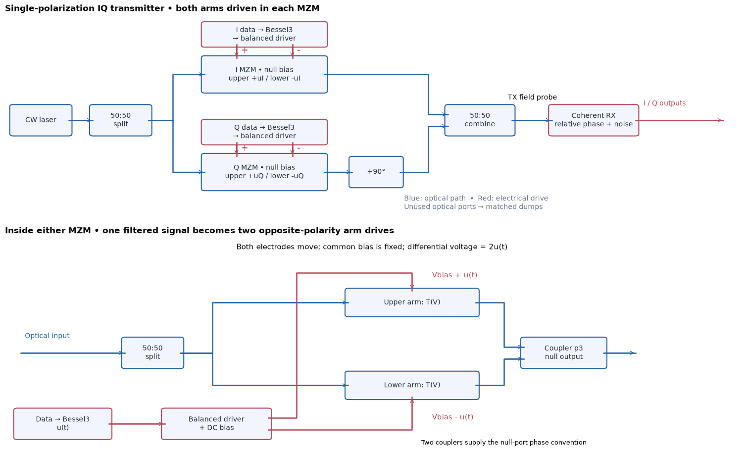
This tutorial connects a laser, couplers, four voltage-controlled optical arms, balanced electrical drivers and a coherent receiver into one complex Circulax circuit. We build one phase shifter, reuse it in a push-pull Mach–Zehnder modulator (MZM), and connect two MZMs as an IQ transmitter. The constellations come from circuit ports.
The goal is to distinguish static optical nonlinearity, bandwidth-induced intersymbol interference (ISI) and receiver impairments. We use one polarization, 56 Gbaud data and 35 GHz third-order Bessel drivers. All component definitions, netlists, random trajectories and plots are embedded here. No PDK, helper module or external data is required.
Environment and scope¤
Use Python 3.12 or later and a Circulax environment with Jupyter. The numerical APIs below were tested with the source checkout c21ba283e57830f0d2bc9f1232ddce7a387dce63, JAX 0.7.2, Diffrax 0.7.2 and KLUJAX 0.5.3. To install that source revision into a virtual environment:
python -m pip install "circulax @ git+https://github.com/gdsfactory/circulax.git@c21ba283e57830f0d2bc9f1232ddce7a387dce63" ipykernel nbconvert
Save this notebook anywhere and run every cell in order. For a short smoke run, set CIRCULAX_NOTEBOOK_CI=1. Parameters are synthetic and illustrative, not a foundry model. The first optical arm is explicitly instantaneous and lumped: no junction capacitance, electrode propagation, optical transit time or dispersion. The public phase_shifter_factory is the next step for a delayed arm; its transit delay would need to be included in the timing reference.
The receiver is an ideal matched field sensor with additive equivalent baseband noise and relative laser/local-oscillator phase noise. It is not a photodiode/TIA implementation. There is no carrier-tracking or adaptive equalization.
# Copyright 2026 Circulax contributors
import os
from dataclasses import dataclass, replace

import jax
import jax.numpy as jnp
import matplotlib.pyplot as plt
import numpy as np
from diffrax import SaveAt
from IPython.display import Markdown
from IPython.display import display as show_markdown
from matplotlib.patches import FancyArrowPatch, FancyBboxPatch
from scipy import signal

from circulax import compile_circuit
from circulax.components import Bessel3
from circulax.components.base_component import component, source
from circulax.components.electronic import VCVS, WAVE_PWL, Resistor, VoltageSource, WaveformVoltageSource
from circulax.components.photonic import DirectionalCoupler, OpticalSource
from circulax.solvers import TrapVectorizedTransientSolver

jax.config.update("jax_enable_x64", True)
plt.rcParams.update({"font.family": "DejaVu Sans", "font.size": 10, "figure.facecolor": "white"})


@dataclass(frozen=True)
class Settings:
    baud: float = 56e9
    bandwidth: float = 35e9
    symbols: int = 1024
    samples_per_ui: int = 32
    warmup: int = 24
    bias: float = -1.5
    swing: float = 1.0  # peak excursion PER ARM (not differential Vpp)
    wavelength_nm: float = 1310.0
    length_um: float = 1000.0
    phase_slope: float = 0.95  # rad/V at the 1 mm, 1310 nm reference geometry
    quadratic: float = 0.28  # rad/V² per arm
    cubic: float = -0.12  # rad/V³ per arm
    loss0: float = 2.0  # total arm loss in dB at bias
    loss1: float = 0.65  # dB/V
    loss2: float = 0.30  # dB/V²
    power: float = 1e-3  # launched laser power in W
    jitter_rms_ui: float = 0.08  # receiver sampling clock only
    reference_rx_power: float = 100e-6  # fixed reference for equivalent receiver noise
    reference_snr_db: float = 22.0
    noise_bandwidth: float = 0.7 * 56e9  # two-sided baseband support: |f| <= this value
    noise_grid_per_ui: int = 8  # independent of the circuit solver time step
    relative_linewidth: float = 500e3  # sum of independent TX/LO Lorentzian linewidths, Hz
    data_seed: int = 23
    noise_seed: int = 101
    phase_seed: int = 202
    jitter_seed: int = 409


cfg = Settings()
if os.environ.get("CIRCULAX_NOTEBOOK_CI") == "1":
    cfg = replace(cfg, symbols=128)
print(f"{cfg.baud / 1e9:g} Gbaud, {cfg.bandwidth / 1e9:g} GHz Bessel3, {cfg.symbols} symbols")
print(f"Sampling jitter {cfg.jitter_rms_ui:g} UI = {cfg.jitter_rms_ui / cfg.baud * 1e12:.2f} ps RMS")
print(
    f"Fixed RX noise power {cfg.reference_rx_power / 10 ** (cfg.reference_snr_db / 10) * 1e6:.3f} µW; relative linewidth {cfg.relative_linewidth / 1e3:g} kHz"
)
56 Gbaud, 35 GHz Bessel3, 1024 symbols
Sampling jitter 0.08 UI = 1.43 ps RMS
Fixed RX noise power 0.631 µW; relative linewidth 500 kHz
1. Read the topology and voltage conventions¤
Each sub-MZM has two driven arms. The I branch receives \(V_b+u_I(t)\) and \(V_b-u_I(t)\); Q receives \(V_b+u_Q(t)\) and \(V_b-u_Q(t)\). One Bessel output feeds two ideal VCVSs with gains +1 and −1, referenced to a shared DC bias. At the default 1 V per-arm peak excursion, each arm has 2 V peak-to-peak swing; the differential arm voltage has 4 V peak-to-peak swing.
DirectionalCoupler has bar coefficient \(t=1/\sqrt2\) and cross coefficient \(j/\sqrt2\). Two such couplers select a null output for equal arm transfers at port p3. The outer Q phase trim is +90°, and the outer combiner's selected port is p4. These choices include the couplers' own phases and yield the I/Q convention derived below. All unused optical ports have matched 1 Ω loads; the receiver input is also matched. Blue paths are optical; red paths are electrical.
2. Author a voltage-controlled optical component¤
Let \(x=V_\mathrm{anode}-V_\mathrm{cathode}-V_b\). The material law is
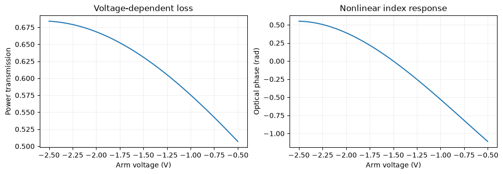
The coefficients describe a reference arm of \(L_0=1000\) µm at \(\lambda_0=1310\) nm. They define a fixed voltage-to-index law: the actual phase then scales as \(L/\lambda\), and total loss in dB scales as \(L/L_0\). Phase is relative to the common carrier phase. The nonlinear flags below switch index curvature and voltage-dependent loss separately. The even phase term changes common phase; the odd term changes differential phase.
A component returns current/field-flow residuals and storage terms. This reciprocal matched optical arm uses incident-wave states a1 and a2; outgoing waves are b1=T*a2, b2=T*a1. At either optical port, field = incident + outgoing and flow = incident − outgoing, with normalized optical impedance 1 Ω. The electrical electrodes are ideal unloaded voltage controls. An empty storage dictionary means this arm adds no dynamics; driver memory is introduced by Bessel3.
def arm_transfer(
    voltage,
    *,
    bias=-1.5,
    phase_slope=0.95,
    quadratic=0.28,
    cubic=-0.12,
    loss0=2.0,
    loss1=0.65,
    loss2=0.30,
    nonlinear=0.0,
    variable_loss=0.0,
    length_um=1000.0,
    wavelength_nm=1310.0,
):
    x = voltage - bias
    phase_law = phase_slope * x + nonlinear * (quadratic * x**2 + cubic * x**3)
    # Convert reference-device phase coefficients to a geometry-independent index law.
    delta_neff = 1310.0 / (2 * jnp.pi * 1000.0 * 1e3) * phase_law
    phase = 2 * jnp.pi * length_um * 1e3 / wavelength_nm * delta_neff
    loss_db = length_um / 1000.0 * (loss0 + variable_loss * (loss1 * x + loss2 * x**2))
    return 10 ** (-loss_db / 20) * jnp.exp(-1j * phase)


@component(ports=("anode", "cathode", "o1", "o2"), states=("a1", "a2"), holomorphic=False)
def LumpedPhaseShifter(  # noqa: N802, PLR0917
    signals,
    bias=-1.5,
    phase_slope=0.95,
    quadratic=0.28,
    cubic=-0.12,
    loss0=2.0,
    loss1=0.65,
    loss2=0.30,
    nonlinear=0.0,
    variable_loss=0.0,
    length_um=1000.0,
    wavelength_nm=1310.0,
):
    voltage = jnp.real(signals.anode - signals.cathode)
    transfer = arm_transfer(
        voltage,
        bias=bias,
        phase_slope=phase_slope,
        quadratic=quadratic,
        cubic=cubic,
        loss0=loss0,
        loss1=loss1,
        loss2=loss2,
        nonlinear=nonlinear,
        variable_loss=variable_loss,
        length_um=length_um,
        wavelength_nm=wavelength_nm,
    )
    b1, b2 = transfer * signals.a2, transfer * signals.a1
    return {
        "anode": 0.0,
        "cathode": 0.0,
        "o1": signals.a1 - b1,
        "o2": signals.a2 - b2,
        "a1": signals.o1 - signals.a1 - b1,
        "a2": signals.o2 - signals.a2 - b2,
    }, {}


@component(ports=("p1", "p2"), states=("a1", "a2"), holomorphic=True)
def PhaseTrim(signals, phase=0.0):  # noqa: N802
    transfer = jnp.exp(1j * phase)
    b1, b2 = transfer * signals.a2, transfer * signals.a1
    return {
        "p1": signals.a1 - b1,
        "p2": signals.a2 - b2,
        "a1": signals.p1 - signals.a1 - b1,
        "a2": signals.p2 - signals.a2 - b2,
    }, {}


def arm_settings(cfg, nonlinear=0.0, variable_loss=0.0):
    names = ("bias", "phase_slope", "quadratic", "cubic", "loss0", "loss1", "loss2", "length_um", "wavelength_nm")
    return {**{name: getattr(cfg, name) for name in names}, "nonlinear": nonlinear, "variable_loss": variable_loss}


models = {
    "R": Resistor,
    "laser": OpticalSource,
    "V": VoltageSource,
    "drive": WaveformVoltageSource,
    "filter": Bessel3,
    "vcvs": VCVS,
    "arm": LumpedPhaseShifter,
    "trim": PhaseTrim,
    "coupler": DirectionalCoupler,
}
Check one component before assembling the modulator¤
Connect a matched laser → phase shifter → matched load, plus a DC electrode source. The laser source field is \(2\sqrt{P_\mathrm{in}}\) before its 1 Ω series matching resistance, so the incident field is \(\sqrt{P_\mathrm{in}}\). Sweep the actual circuit's electrode voltage and compare its output with the independently evaluated transfer law.
arm_net = {
    "instances": {
        "GND": {"component": "ground"},
        "LASER": {"component": "laser", "settings": {"power": 4 * cfg.power}},
        "MATCH": {"component": "R", "settings": {"R": 1.0}},
        "PS": {"component": "arm", "settings": arm_settings(cfg, 1.0, 1.0)},
        "BIAS": {"component": "V", "settings": {"V": cfg.bias}},
        "LOAD": {"component": "R", "settings": {"R": 1.0}},
    },
    "connections": {
        "LASER,p1": "MATCH,p1",
        "MATCH,p2": "PS,o1",
        "PS,o2": "LOAD,p1",
        "BIAS,p1": "PS,anode",
        "GND,p1": ("LASER,p2", "PS,cathode", "BIAS,p2", "LOAD,p2"),
    },
    "ports": {"output": "LOAD,p1"},
}
arm_circuit = compile_circuit(arm_net, models, is_complex=True, backend="dense", g_leak=0.0)
voltages = jnp.linspace(cfg.bias - cfg.swing, cfg.bias + cfg.swing, 101)
arm_fields = np.asarray(arm_circuit.port(arm_circuit.dc(params={"BIAS.V": voltages}), "output"))
expected_arm = np.sqrt(cfg.power) * np.asarray(arm_transfer(voltages, **arm_settings(cfg, 1.0, 1.0)))
np.testing.assert_allclose(arm_fields, expected_arm, atol=1e-10, rtol=1e-7)
fig, axes = plt.subplots(1, 2, figsize=(10, 3.4), layout="constrained")
axes[0].plot(voltages, abs(arm_fields) ** 2 / cfg.power)
axes[0].set(xlabel="Arm voltage (V)", ylabel="Power transmission", title="Voltage-dependent loss")
axes[1].plot(voltages, np.unwrap(np.angle(arm_fields)))
axes[1].set(xlabel="Arm voltage (V)", ylabel="Optical phase (rad)", title="Nonlinear index response")
for ax in axes:
    ax.grid(alpha=0.2)
plt.show()
3. Build one MZM, then reuse it twice¤
For the chosen two-coupler null port,
At the reference geometry, linear index and constant loss give \(D(u)=10^{-\ell_0/20}\sin(ku)\). Thus even a linear index law produces a nonlinear MZM field. The following netlist exposes optical input/output, the two electrical arm controls and two dump-monitor ports. Compiling it creates a reusable hierarchical component. The dump loads keep unselected optical outputs matched.
def mzm_netlist(cfg):
    return {
        "instances": {
            "GND": {"component": "ground"},
            "SPLIT": {"component": "coupler"},
            "COMBINE": {"component": "coupler"},
            "UPPER": {"component": "arm", "settings": arm_settings(cfg)},
            "LOWER": {"component": "arm", "settings": arm_settings(cfg)},
            "DUMP_IN": {"component": "R", "settings": {"R": 1.0}},
            "DUMP_OUT": {"component": "R", "settings": {"R": 1.0}},
        },
        "connections": {
            "SPLIT,p2": "DUMP_IN,p1",
            "SPLIT,p3": "UPPER,o1",
            "SPLIT,p4": "LOWER,o1",
            "UPPER,o2": "COMBINE,p1",
            "LOWER,o2": "COMBINE,p2",
            "COMBINE,p4": "DUMP_OUT,p1",
            "GND,p1": ("UPPER,cathode", "LOWER,cathode", "DUMP_IN,p2", "DUMP_OUT,p2"),
        },
        "ports": {
            "optical_in": "SPLIT,p1",
            "optical_out": "COMBINE,p3",
            "upper_drive": "UPPER,anode",
            "lower_drive": "LOWER,anode",
            "dump_in": "DUMP_IN,p1",
            "dump_out": "DUMP_OUT,p1",
        },
    }


mzm_model = compile_circuit(mzm_netlist(cfg), models, is_complex=True, g_leak=0.0)
models["mzm"] = mzm_model
print("Reusable MZM ports:", list(mzm_netlist(cfg)["ports"]))
Reusable MZM ports: ['optical_in', 'optical_out', 'upper_drive', 'lower_drive', 'dump_in', 'dump_out']
4. Define stochastic trajectories at the receiver boundary¤
A clean, noiseless transmitter constellation is useful: static nonlinearity moves centroids, while bandwidth adds deterministic pattern dependence. Sampling jitter gives approximately \(\delta E=\dot E\,\delta t\) and has little effect on flat portions of a symbol. These effects do not produce the rounded clouds caused by additive noise.
We therefore connect an explicit ideal coherent receiver with normalized outputs in \(\sqrt{\mathrm W}\):
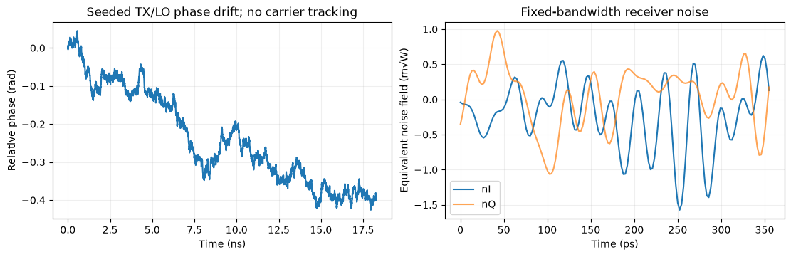
- Additive noise: independent zero-mean quadratures, with total noise power \(P_n=P_\mathrm{ref}/10^{\mathrm{SNR}_{ref}/10}\). Here the fixed reference is 100 µW and 22 dB, not the power of each case. Lower signal power therefore retains its SNR penalty. The equivalent noise has rectangular spectral support \(|f|\le B_n\) on a fixed 8-samples/UI grid. It is generated once and normalized on that grid. The receiver's signal extraction is otherwise ideal; this is an equivalent input noise model, not a full filtered detector model.
- Relative TX/LO phase noise: a Wiener trajectory with \(\mathrm{Var}(\theta_{k+1}-\theta_k)=2\pi\Delta\nu_\mathrm{rel}\Delta t\). For independent Lorentzian lasers, \(\Delta\nu_\mathrm{rel}\) is the sum of their linewidths. The trajectory is fixed for all comparisons; there is no carrier tracking.
- Sampling-clock jitter: applied later as \(t_n=t_{n,0}+\delta t_n\), with \(\delta t_n\sim\mathcal N(0,(\sigma_\mathrm{UI}/R_s)^2)\) and a shared I/Q clock. This is separate from transmitter edge jitter, which is not included.
Random arrays are generated before circuit compilation. The receiver interpolates these deterministic arrays during solving, so Newton iterations always see the same forcing at a given time. Its noise/phase grid does not change when the circuit step is refined.
def receiver_trajectories(cfg):
    count = cfg.symbols * cfg.noise_grid_per_ui + 1
    times = np.arange(count) / (cfg.noise_grid_per_ui * cfg.baud)
    dt = times[1] - times[0]
    assert 0 < cfg.noise_bandwidth < 0.5 / dt
    white = np.random.default_rng(cfg.noise_seed).normal(size=(count, 2))
    spectrum = np.fft.rfft(white, axis=0)
    frequencies = np.fft.rfftfreq(count, dt)
    spectrum[frequencies > cfg.noise_bandwidth] = 0
    spectrum[0] = 0  # zero mean over the finite periodic noise record
    noise = np.fft.irfft(spectrum, n=count, axis=0)
    noise_power = cfg.reference_rx_power / 10 ** (cfg.reference_snr_db / 10)
    noise *= np.sqrt(noise_power / 2) / np.std(noise, axis=0)
    increments = np.random.default_rng(cfg.phase_seed).normal(0, np.sqrt(2 * np.pi * cfg.relative_linewidth * dt), count - 1)
    phase = np.r_[0.0, np.cumsum(increments)]
    return {"times": times, "noise": noise, "phase": phase, "noise_power": noise_power}


trajectories = receiver_trajectories(cfg)


@source(ports=("optical", "I", "Q"), states=("i_I", "i_Q"), holomorphic=False)
def CoherentReceiver(  # noqa: N802, PLR0917
    signals, t, noise_on=1.0, phase_on=1.0, grid_t=(0.0, 1.0), noise_i=(0.0, 0.0), noise_q=(0.0, 0.0), theta=(0.0, 0.0)
):
    rotation = phase_on * jnp.interp(t, grid_t, theta)
    noise = noise_on * (jnp.interp(t, grid_t, noise_i) + 1j * jnp.interp(t, grid_t, noise_q))
    z = signals.optical * jnp.exp(1j * rotation) + noise
    return {
        "optical": signals.optical,  # matched 1-ohm optical load
        "I": signals.i_I,
        "Q": signals.i_Q,
        "i_I": signals.I - jnp.real(z),
        "i_Q": signals.Q - jnp.imag(z),
    }, {}


models["receiver"] = CoherentReceiver
print(f"Noise grid: {cfg.noise_grid_per_ui} samples/UI, band limit {cfg.noise_bandwidth / 1e9:g} GHz")
Noise grid: 8 samples/UI, band limit 39.2 GHz
5. Connect the complete IQ circuit¤
The source launches \(\sqrt{P_\mathrm{in}}\) after matching. The outer split feeds two instances of our MZM component. With the Q trim at +90° and the selected outer output at p4, the reference transfer is
The 1/2 factor includes the outer splitting and combining. The receiver loads the selected optical output and exposes real I/Q baseband ports. Both optical and electrical domains participate in the same complex solve.
Each independent I/Q bit stream is Gray mapped: QPSK uses ±1 per axis; 16-QAM maps 00,01,11,10 to −1, −1/3, +1/3, +1. Each source ramps over 0.1 UI before holding its symbol level. The filters are genuine third-order Bessel blocks normalized to their −3 dB cutoff, not cascaded identical RC filters.
def symbol_data(order, cfg):
    bits = np.random.default_rng(cfg.data_seed).integers(0, 2, (cfg.symbols, 2, 1 if order == 4 else 2))
    axis = np.linspace(-1, 1, int(np.sqrt(order)))
    indices = bits[..., 0] if order == 4 else np.array([0, 1, 3, 2])[2 * bits[..., 0] + bits[..., 1]]
    return axis[indices], indices[:, 0] * len(axis) + indices[:, 1]


def iq_netlist(levels, cfg, trajectories):
    instances = {
        "GND": {"component": "ground"},
        "LASER": {"component": "laser", "settings": {"power": 4 * cfg.power}},
        "MATCH": {"component": "R", "settings": {"R": 1.0}},
        "BIAS": {"component": "V", "settings": {"V": cfg.bias}},
        "SPLIT": {"component": "coupler"},
        "COMBINE": {"component": "coupler"},
        "I_MZM": {"component": "mzm"},
        "Q_MZM": {"component": "mzm"},
        "Q_TRIM": {"component": "trim", "settings": {"phase": np.pi / 2}},
        "RX": {
            "component": "receiver",
            "settings": {
                "grid_t": jnp.asarray(trajectories["times"]),
                "noise_i": jnp.asarray(trajectories["noise"][:, 0]),
                "noise_q": jnp.asarray(trajectories["noise"][:, 1]),
                "theta": jnp.asarray(trajectories["phase"]),
            },
        },
    }
    connections = {
        "LASER,p1": "MATCH,p1",
        "MATCH,p2": "SPLIT,p1",
        "LASER,p2": "GND,p1",
        "BIAS,p2": "GND,p1",
        "SPLIT,p3": "I_MZM,optical_in",
        "SPLIT,p4": "Q_MZM,optical_in",
        "I_MZM,optical_out": "COMBINE,p1",
        "Q_MZM,optical_out": "Q_TRIM,p1",
        "Q_TRIM,p2": "COMBINE,p2",
        "COMBINE,p4": "RX,optical",
    }
    ports = {"tx": "RX,optical", "rx_i": "RX,I", "rx_q": "RX,Q"}
    for name, port in (("DUMP_IN", "SPLIT,p2"), ("DUMP_OUT", "COMBINE,p3")):
        instances[name] = {"component": "R", "settings": {"R": 1.0}}
        connections[port] = f"{name},p1"
        connections[f"{name},p2"] = "GND,p1"
        ports[name] = f"{name},p1"
    boundaries = np.arange(len(levels)) / cfg.baud
    knots = np.r_[np.column_stack((boundaries, boundaries + 0.1 / cfg.baud)).ravel(), len(levels) / cfg.baud]
    for k, branch in enumerate(("I", "Q")):
        values = cfg.swing * levels[:, k]
        previous = np.r_[values[0], values[:-1]]
        instances[f"{branch}_DATA"] = {
            "component": "drive",
            "settings": {
                "kind": WAVE_PWL,
                "pwl_t": jnp.asarray(knots),
                "pwl_v": jnp.asarray(np.r_[np.column_stack((previous, values)).ravel(), values[-1]]),
            },
        }
        instances[f"{branch}_FILTER"] = {"component": "filter", "settings": {"f3db": cfg.bandwidth}}
        connections[f"{branch}_DATA,p1"] = f"{branch}_FILTER,inp"
        connections[f"{branch}_DATA,p2"] = "GND,p1"
        for arm, gain, electrode in (("UP", 1.0, "upper_drive"), ("LOW", -1.0, "lower_drive")):
            name = f"{branch}_{arm}"
            instances[name] = {"component": "vcvs", "settings": {"A": gain}}
            connections[f"{name},ctrl_p"] = f"{branch}_FILTER,out"
            connections[f"{name},ctrl_m"] = "GND,p1"
            connections[f"{name},out_m"] = "BIAS,p1"
            connections[f"{name},out_p"] = f"{branch}_MZM,{electrode}"
            ports[name] = f"{branch}_MZM,{electrode}"
        ports[f"{branch}_drive"] = f"{branch}_FILTER,out"
        # Read monitor ports exposed by the reusable MZM interface.
        for dump in ("DUMP_IN", "DUMP_OUT"):
            ports[f"{branch}_{dump}"] = f"{branch}_MZM,{dump.lower()}"
    return {"instances": instances, "connections": connections, "ports": ports}


levels, labels = symbol_data(16, cfg)
netlist = iq_netlist(levels, cfg, trajectories)
iq_circuit = compile_circuit(netlist, models, is_complex=True, g_leak=0.0)
print(f"Connected IQ circuit: {iq_circuit.sys_size} unknowns; {len(netlist['instances'])} top-level components")
print("I upper-arm connection:", netlist["connections"]["I_UP,out_p"])
print("I lower-arm connection:", netlist["connections"]["I_LOW,out_p"])
Connected IQ circuit: 60 unknowns; 20 top-level components
I upper-arm connection: I_MZM,upper_drive
I lower-arm connection: I_MZM,lower_drive
6. Validate the connected circuit at DC¤
The analytical expression below is a reference, not the source of the plotted circuit fields. Sweep the actual connected circuit through every static 16-QAM state for three optical laws. At DC the filters have unity gain. Source dc overrides select operating-point voltages without changing the transient PWL waveforms. The receiver impairments are disabled for these checks.
Hierarchy parameter paths such as I_MZM~UPPER.nonlinear configure the individual arm components. Check the absolute complex field, both opposite-polarity voltages, and passive optical power at the selected output plus all dumps.
CASES = {"Linear index": (0.0, 0.0), "Nonlinear index": (1.0, 0.0), "Nonlinear index + loss": (1.0, 1.0)}
DUMP_PORTS = ["DUMP_IN", "DUMP_OUT", "I_DUMP_IN", "I_DUMP_OUT", "Q_DUMP_IN", "Q_DUMP_OUT"]


def optical_params(nonlinear, variable_loss):
    return {
        f"{branch}_MZM~{arm}.{name}": value
        for branch in ("I", "Q")
        for arm in ("UPPER", "LOWER")
        for name, value in (("nonlinear", nonlinear), ("variable_loss", variable_loss))
    }


def analytic_field(drives, cfg, nonlinear, variable_loss):
    upper = np.asarray(arm_transfer(cfg.bias + drives, **arm_settings(cfg, nonlinear, variable_loss)))
    lower = np.asarray(arm_transfer(cfg.bias - drives, **arm_settings(cfg, nonlinear, variable_loss)))
    d = (lower - upper) / (2j)
    return np.sqrt(cfg.power) / 2 * (d[..., 0] + 1j * d[..., 1])


static_grid = np.array([(i, q) for i in (-1, -1 / 3, 1 / 3, 1) for q in (-1, -1 / 3, 1 / 3, 1)])
static_results = {}
for name, (nl, loss) in CASES.items():
    params = {
        **optical_params(nl, loss),
        "RX.noise_on": 0.0,
        "RX.phase_on": 0.0,
        "I_DATA.dc_given": 1.0,
        "Q_DATA.dc_given": 1.0,
        "I_DATA.dc": jnp.asarray(cfg.swing * static_grid[:, 0]),
        "Q_DATA.dc": jnp.asarray(cfg.swing * static_grid[:, 1]),
    }
    dc = iq_circuit.dc(params=params)
    actual = np.asarray(iq_circuit.port(dc, "tx"))
    expected = analytic_field(cfg.swing * static_grid, cfg, nl, loss)
    np.testing.assert_allclose(actual, expected, atol=1e-9, rtol=1e-6)
    for branch in ("I", "Q"):
        upper = np.asarray(iq_circuit.port(dc, branch + "_UP")).real
        lower = np.asarray(iq_circuit.port(dc, branch + "_LOW")).real
        np.testing.assert_allclose(upper + lower, 2 * cfg.bias, atol=1e-9)
    observed = abs(actual) ** 2 + sum(abs(np.asarray(iq_circuit.port(dc, port))) ** 2 for port in DUMP_PORTS)
    assert np.max(observed) <= cfg.power * (1 + 1e-6)
    if loss == 0.0:
        np.testing.assert_allclose(observed, cfg.power * 10 ** (-cfg.loss0 * (cfg.length_um / 1000.0) / 10), rtol=1e-6)
    static_results[name] = actual
print("All 48 connected static symbol states agree with the analytical field reference.")
All 48 connected static symbol states agree with the analytical field reference.
7. Run the connected transient and read circuit ports¤
A sparse trapezoidal solver advances the Bessel states while solving all optical/electrical constraints. Only the plotted ports are saved; the full circuit state remains inside the solver. Use a fixed step of 1/32 UI and discard 24 warmup symbols plus four end symbols.
The nominal receiver sampling delay is the Bessel DC group delay plus half the source ramp. It is shared by every optical law, with no timing optimization per case. Sampling jitter changes the query times of both receiver quadratures together. One fitted complex gain removes an average phase/amplitude factor; it does not perform carrier tracking, independent I/Q scaling, DC subtraction or equalization.
def align(samples, target):
    gain = np.vdot(target, samples) / np.vdot(target, target)
    values = samples / gain
    evm = np.sqrt(np.mean(abs(values - target) ** 2) / np.mean(abs(target) ** 2))
    return values, evm, gain


def sample_field(times, field, cfg, jitter_rms_ui=0.0):
    if not np.isfinite(jitter_rms_ui) or jitter_rms_ui < 0:
        msg = "Jitter must be finite and nonnegative"
        raise ValueError(msg)
    indices = np.arange(cfg.warmup, cfg.symbols - 4)
    delay = 1.7556723686812106 / (2 * np.pi * cfg.bandwidth) + 0.05 / cfg.baud
    query = (indices + 0.5) / cfg.baud + delay
    query += np.random.default_rng(cfg.jitter_seed).normal(0, jitter_rms_ui / cfg.baud, len(indices))
    if np.any(query < times[0]) or np.any(query > times[-1]):
        msg = "Sampling times leave the record; increase guards or reduce jitter"
        raise ValueError(msg)
    return indices, np.interp(query, times, field.real) + 1j * np.interp(query, times, field.imag)


def receiver_reference(field, times, trajectories, noise_on=1.0, phase_on=1.0):
    theta = np.interp(times, trajectories["times"], trajectories["phase"])
    ni = np.interp(times, trajectories["times"], trajectories["noise"][:, 0])
    nq = np.interp(times, trajectories["times"], trajectories["noise"][:, 1])
    return field * np.exp(1j * phase_on * theta) + noise_on * (ni + 1j * nq)


SAVE_PORTS = ["tx", "rx_i", "rx_q", "I_UP", "I_LOW", "Q_UP", "Q_LOW", "I_drive", "Q_drive", *DUMP_PORTS]


def simulate(circuit, cfg, params=None, resolution=1):
    dt = 1 / (cfg.baud * cfg.samples_per_ui * resolution)
    times = np.arange(cfg.symbols * cfg.samples_per_ui * resolution + 1) * dt
    saved = SaveAt(ts=jnp.asarray(times), fn=lambda _t, y, _args: jnp.stack([circuit.port(y, port) for port in SAVE_PORTS]))
    solution = circuit.transient(
        t0=0.0,
        t1=float(times[-1]),
        dt0=dt,
        params=params,
        saveat=saved,
        transient_solver=TrapVectorizedTransientSolver,
        max_steps=len(times) + 20,
        throw=True,
    )
    values = np.asarray(solution.ys)
    assert np.isfinite(values).all()
    return times, {port: values[:, k] for k, port in enumerate(SAVE_PORTS)}


runs = {}
for order in (4, 16):
    levels, labels = symbol_data(order, cfg)
    circuit = compile_circuit(iq_netlist(levels, cfg, trajectories), models, is_complex=True, g_leak=0.0)
    cases = {}
    for name, (nl, loss) in CASES.items():
        times, traces = simulate(circuit, cfg, optical_params(nl, loss))
        tx, rx = traces["tx"], traces["rx_i"].real + 1j * traces["rx_q"].real
        for branch in ("I", "Q"):
            np.testing.assert_allclose(traces[branch + "_UP"] + traces[branch + "_LOW"], 2 * cfg.bias, atol=1e-8)
        expected = analytic_field(np.column_stack((traces["I_drive"].real, traces["Q_drive"].real)), cfg, nl, loss)
        np.testing.assert_allclose(tx, expected, atol=1e-8, rtol=1e-5)
        np.testing.assert_allclose(rx, receiver_reference(tx, times, trajectories), atol=1e-8, rtol=1e-5)
        total_power = abs(tx) ** 2 + sum(abs(traces[port]) ** 2 for port in DUMP_PORTS)
        assert np.max(total_power) <= cfg.power * (1 + 1e-5)
        idx, tx_samples = sample_field(times, tx, cfg)
        _, rx_samples = sample_field(times, rx, cfg, cfg.jitter_rms_ui)
        target = levels[idx, 0] + 1j * levels[idx, 1]
        tx_values, tx_evm, _ = align(tx_samples, target)
        rx_values, rx_evm, _ = align(rx_samples, target)
        cases[name] = {"traces": traces, "tx_values": tx_values, "tx_evm": tx_evm, "rx_values": rx_values, "rx_evm": rx_evm}
        print(f"{'QPSK' if order == 4 else '16-QAM'} / {name}: TX {100 * tx_evm:.2f}% EVM; RX {100 * rx_evm:.2f}% EVM", flush=True)
    runs[order] = {"times": times, "cases": cases, "target": target, "labels": labels[idx], "levels": levels}
print("All connected transient checks passed: push-pull, field recombination, receiver equation and passive power.")
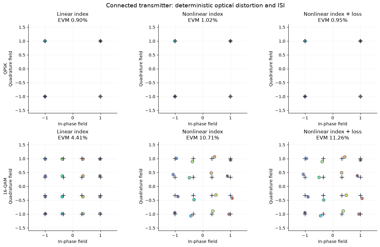
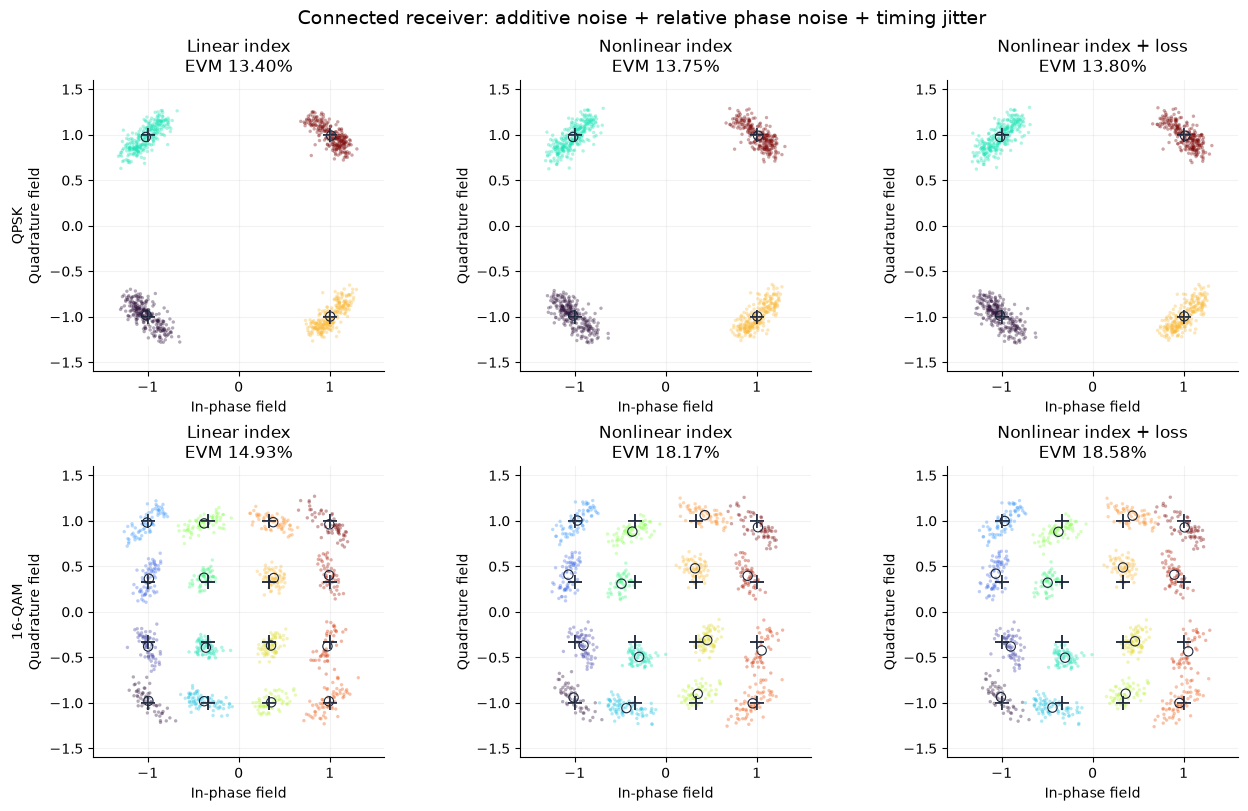
QPSK / Linear index: TX 0.90% EVM; RX 13.40% EVM


QPSK / Nonlinear index: TX 1.02% EVM; RX 13.75% EVM


QPSK / Nonlinear index + loss: TX 0.95% EVM; RX 13.80% EVM


16-QAM / Linear index: TX 4.41% EVM; RX 14.93% EVM


16-QAM / Nonlinear index: TX 10.71% EVM; RX 18.17% EVM


16-QAM / Nonlinear index + loss: TX 11.26% EVM; RX 18.58% EVM


All connected transient checks passed: push-pull, field recombination, receiver equation and passive power.
8. Compare transmitter distortion with receiver clouds¤
Crosses are ideal symbols; circles are cluster centroids; colours identify transmitted classes. Axes and normalization conventions are shared. The first figure uses the transmitter optical field with no receiver noise or clock jitter. The second uses the connected receiver outputs, including relative phase noise, additive noise and sampling jitter.
The noise power is identical across all cases, rather than rescaled to each case's signal power. EVM includes all remaining errors after one complex gain fit, using known transmitted symbols. It is not a BER estimate. QPSK has only one magnitude per axis and can hide symmetric static nonlinearity. The multiple magnitudes in 16-QAM reveal amplitude compression and amplitude-dependent phase.
for receiver in (False, True):
    fig, axes = plt.subplots(2, 3, figsize=(13, 8), layout="constrained")
    key = "rx" if receiver else "tx"
    for row, order in enumerate((4, 16)):
        run = runs[order]
        for ax, (name, case) in zip(axes[row], run["cases"].items(), strict=True):
            constellation(ax, case[key + "_values"], run["target"], run["labels"], f"{name}\nEVM {100 * case[key + '_evm']:.2f}%")
        axes[row, 0].set_ylabel(("QPSK" if order == 4 else "16-QAM") + "\nQuadrature field")
    title = (
        "Connected receiver: additive noise + relative phase noise + timing jitter"
        if receiver
        else "Connected transmitter: deterministic optical distortion and ISI"
    )
    fig.suptitle(title, fontsize=14)
    plt.show()
9. Attribute the cloud shape to an impairment¤
Use the same nonlinear-index/loss circuit field and the same receiver trajectories with one impairment enabled at a time. For these ablations we reuse the receiver equation after solving; the all-on equation was verified sample-by-sample against the connected CoherentReceiver outputs above. This saves redundant circuit solves because the matched receiver does not feed its baseband noise back into the transmitter.
Additive noise gives approximately rounded clouds. Relative phase noise produces angular spreading and drift across the finite record; its EVM depends on record duration and the absence of carrier tracking. Sampling-clock jitter follows the local waveform slope and often produces directed tails. These EVM contributions do not add arithmetically: correlated errors may partially cancel. The MZM sine can also reduce sensitivity to voltage errors at outer levels, so a more linear static transfer is not necessarily a lower bound on dynamic EVM.
ablations = {
    "No receiver impairments": (0.0, 0.0, 0.0),
    "Additive noise only": (1.0, 0.0, 0.0),
    "Relative phase only": (0.0, 1.0, 0.0),
    "Timing jitter only": (0.0, 0.0, cfg.jitter_rms_ui),
    "All receiver impairments": (1.0, 1.0, cfg.jitter_rms_ui),
}
fig, axes = plt.subplots(2, 5, figsize=(19, 8), layout="constrained")
rows = ["| Format | Receiver impairments | EVM |", "|---|---|---:|"]
for row, order in enumerate((4, 16)):
    run = runs[order]
    tx = run["cases"]["Nonlinear index + loss"]["traces"]["tx"]
    for ax, (name, (noise, phase, jitter)) in zip(axes[row], ablations.items(), strict=True):
        field = receiver_reference(tx, run["times"], trajectories, noise, phase)
        _, sampled = sample_field(run["times"], field, cfg, jitter)
        values, evm, _ = align(sampled, run["target"])
        constellation(ax, values, run["target"], run["labels"], f"{name}\nEVM {100 * evm:.2f}%")
        rows.append(f"| {'QPSK' if order == 4 else '16-QAM'} | {name} | {100 * evm:.2f}% |")
    axes[row, 0].set_ylabel(("QPSK" if order == 4 else "16-QAM") + "\nQuadrature field")
fig.suptitle("Impairment attribution • nonlinear index + voltage-dependent loss", fontsize=15)
plt.show()
show_markdown(Markdown("\n".join(rows)))

fig, axes = plt.subplots(1, 2, figsize=(11, 3.5), layout="constrained")
axes[0].plot(trajectories["times"] * 1e9, trajectories["phase"])
axes[0].set(xlabel="Time (ns)", ylabel="Relative phase (rad)", title="Seeded TX/LO phase drift; no carrier tracking")
axes[1].plot(trajectories["times"][:160] * 1e12, trajectories["noise"][:160, 0] * 1e3, label="nI")
axes[1].plot(trajectories["times"][:160] * 1e12, trajectories["noise"][:160, 1] * 1e3, label="nQ", alpha=0.7)
axes[1].set(xlabel="Time (ps)", ylabel="Equivalent noise field (m√W)", title="Fixed-bandwidth receiver noise")
for ax in axes:
    ax.grid(alpha=0.2)
axes[1].legend()
plt.show()
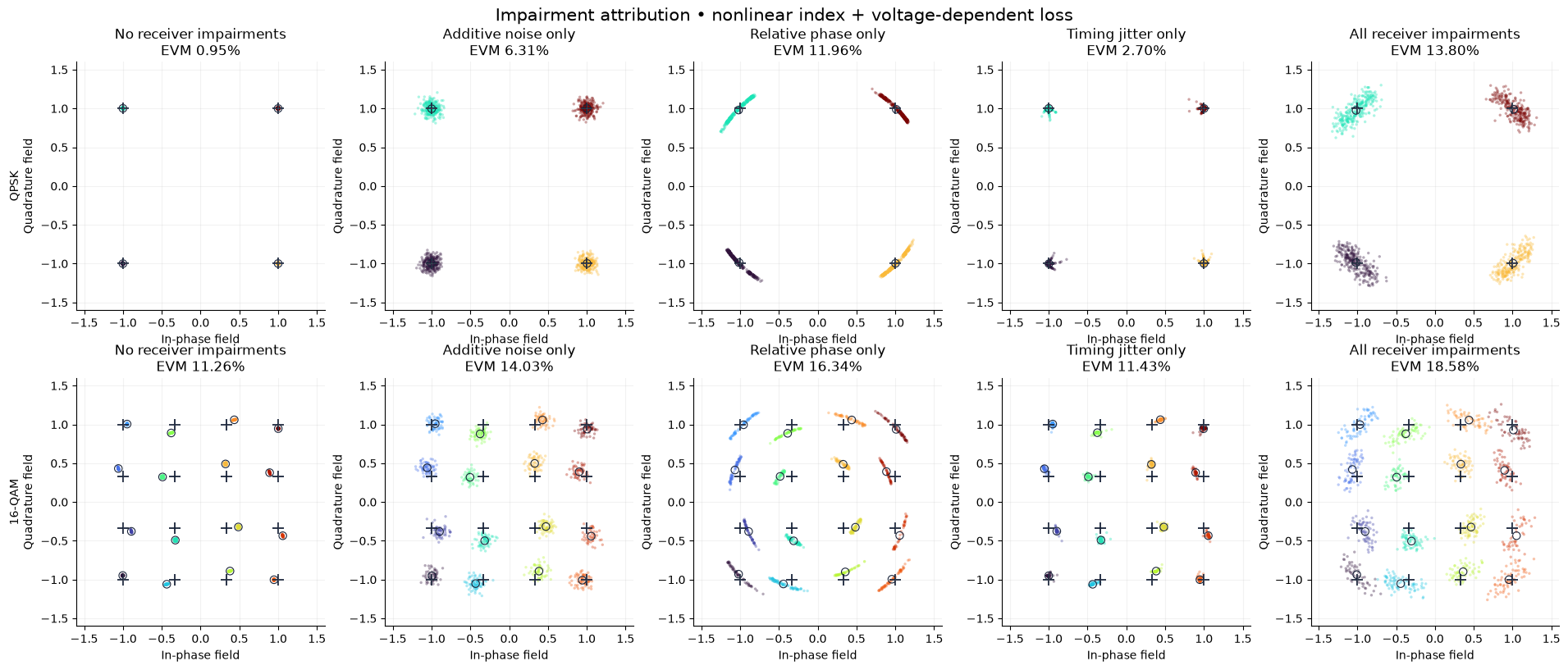
| Format | Receiver impairments | EVM |
|---|---|---|
| QPSK | No receiver impairments | 0.95% |
| QPSK | Additive noise only | 6.31% |
| QPSK | Relative phase only | 11.96% |
| QPSK | Timing jitter only | 2.70% |
| QPSK | All receiver impairments | 13.80% |
| 16-QAM | No receiver impairments | 11.26% |
| 16-QAM | Additive noise only | 14.03% |
| 16-QAM | Relative phase only | 16.34% |
| 16-QAM | Timing jitter only | 11.43% |
| 16-QAM | All receiver impairments | 18.58% |
10. Inspect actual voltages and optical power¤
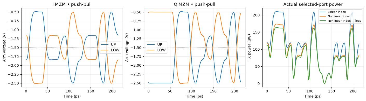
These traces come from the circuit ports. Both arms of both MZMs move with equal and opposite excursions around the same bias. The physical output-power table is shown before any fitted constellation gain: normalization must not hide useful-power and SNR tradeoffs.
run = runs[16]
case = run["cases"]["Nonlinear index + loss"]
a = cfg.warmup * cfg.samples_per_ui
b = a + 12 * cfg.samples_per_ui
ps = (run["times"][a:b] - run["times"][a]) * 1e12
fig, axes = plt.subplots(1, 3, figsize=(14, 3.8), layout="constrained")
for ax, branch in zip(axes[:2], ("I", "Q"), strict=True):
    for arm in ("UP", "LOW"):
        ax.plot(ps, case["traces"][branch + "_" + arm][a:b].real, label=arm)
    ax.axhline(cfg.bias, color="grey", ls=":", lw=1)
    ax.set(xlabel="Time (ps)", ylabel="Arm voltage (V)", title=branch + " MZM • push-pull")
    ax.legend()
for name, values in run["cases"].items():
    axes[2].plot(ps, abs(values["traces"]["tx"][a:b]) ** 2 * 1e6, label=name)
axes[2].set(xlabel="Time (ps)", ylabel="TX power (µW)", title="Actual selected-port power")
axes[2].legend(fontsize=8)
for ax in axes:
    ax.grid(alpha=0.2)
plt.show()
rows = ["| Format | Optical law | Mean TX power (µW) | TX EVM | RX EVM |", "|---|---|---:|---:|---:|"]
for order, run in runs.items():
    for name, case in run["cases"].items():
        field = case["traces"]["tx"][cfg.warmup * cfg.samples_per_ui : -4 * cfg.samples_per_ui]
        rows.append(
            f"| {'QPSK' if order == 4 else '16-QAM'} | {name} | {np.mean(abs(field) ** 2) * 1e6:.2f} | {100 * case['tx_evm']:.2f}% | {100 * case['rx_evm']:.2f}% |"
        )
show_markdown(Markdown("\n".join(rows)))
| Format | Optical law | Mean TX power (µW) | TX EVM | RX EVM |
|---|---|---|---|---|
| QPSK | Linear index | 162.78 | 0.90% | 13.40% |
| QPSK | Nonlinear index | 136.19 | 1.02% | 13.75% |
| QPSK | Nonlinear index + loss | 129.28 | 0.95% | 13.80% |
| 16-QAM | Linear index | 94.78 | 4.41% | 14.93% |
| 16-QAM | Nonlinear index | 81.77 | 10.71% | 18.17% |
| 16-QAM | Nonlinear index + loss | 78.49 | 11.26% | 18.58% |
11. Static calibration and the drive–power tradeoff¤
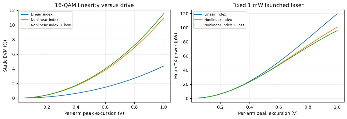
An inverse-sine electrical map \(u=\arcsin[\sin(k_\mathrm{eff}A)d]/k_\mathrm{eff}\), where \(k_\mathrm{eff}=k(L/L_0)(\lambda_0/\lambda)\), exactly linearizes the static linear-index MZM field on the monotonic branch \(|k_\mathrm{eff}A|<\pi/2\). It does not remove nonlinear material phase/loss or dynamic ISI. Check this on the actual connected circuit, then sweep the per-arm drive using the validated analytical static reference. This final sweep isolates static distortion from receiver impairments.
effective_k = cfg.phase_slope * (cfg.length_um / 1000.0) * (1310.0 / cfg.wavelength_nm)
assert 0 < effective_k * cfg.swing < np.pi / 2
calibrated = np.arcsin(np.sin(effective_k * cfg.swing) * static_grid) / effective_k
params = {
    **optical_params(0.0, 0.0),
    "RX.noise_on": 0.0,
    "RX.phase_on": 0.0,
    "I_DATA.dc_given": 1.0,
    "Q_DATA.dc_given": 1.0,
    "I_DATA.dc": jnp.asarray(calibrated[:, 0]),
    "Q_DATA.dc": jnp.asarray(calibrated[:, 1]),
}
cal_dc = iq_circuit.dc(params=params)
cal_field = np.asarray(iq_circuit.port(cal_dc, "tx"))
static_target = static_grid[:, 0] + 1j * static_grid[:, 1]
_, cal_evm, _ = align(cal_field, static_target)
assert cal_evm < 1e-7
print(f"Connected inverse-sine static calibration EVM: {100 * cal_evm:.3g}%")
fig, axes = plt.subplots(1, 2, figsize=(11, 3.7), layout="constrained")
swings = np.linspace(0.05, cfg.swing, 60)
for name, (nl, loss) in CASES.items():
    fields = [analytic_field(swing * static_grid, cfg, nl, loss) for swing in swings]
    axes[0].plot(swings, [100 * align(field, static_target)[1] for field in fields], label=name)
    axes[1].plot(swings, [np.mean(abs(field) ** 2) * 1e6 for field in fields], label=name)
axes[0].set(xlabel="Per-arm peak excursion (V)", ylabel="Static EVM (%)", title="16-QAM linearity versus drive")
axes[1].set(xlabel="Per-arm peak excursion (V)", ylabel="Mean TX power (µW)", title=f"Fixed {cfg.power * 1e3:g} mW launched laser")
for ax in axes:
    ax.grid(alpha=0.2)
    ax.legend(fontsize=8)
plt.show()
Connected inverse-sine static calibration EVM: 2.09e-07%
12. Check numerical error separately from physical impairments¤
Compare the actual driver port with an independent SciPy analog Bessel response. Then rerun a short connected IQ circuit with half the time step, using exactly the same noise/phase arrays and fixed sampling-jitter sequence. Check both optical field and receiver samples. Solver refinement must not generate new noise or change its specified bandwidth.
The linear-field sampling test checks jitter units and shared I/Q timing. A zero-impairment receiver must reproduce the TX field. Repeatability is checked using regenerated seeded trajectories.
check_cfg = replace(cfg, symbols=80)
check_levels, _ = symbol_data(16, check_cfg)
check_trajectories = receiver_trajectories(check_cfg)
check_circuit = compile_circuit(iq_netlist(check_levels, check_cfg, check_trajectories), models, is_complex=True, g_leak=0.0)
check_params = optical_params(1.0, 1.0)
t0, coarse = simulate(check_circuit, check_cfg, check_params)
t1, fine = simulate(check_circuit, check_cfg, check_params, resolution=2)
field_change = np.sqrt(np.mean(abs(coarse["tx"] - fine["tx"][::2]) ** 2) / np.mean(abs(fine["tx"][::2]) ** 2))
rx0 = coarse["rx_i"].real + 1j * coarse["rx_q"].real
rx1 = fine["rx_i"].real + 1j * fine["rx_q"].real
_, sampled0 = sample_field(t0, rx0, check_cfg, cfg.jitter_rms_ui)
_, sampled1 = sample_field(t1, rx1, check_cfg, cfg.jitter_rms_ui)
rx_change = np.sqrt(np.mean(abs(sampled0 - sampled1) ** 2) / np.mean(abs(sampled1) ** 2))
assert field_change < 0.01
assert rx_change < 0.01

num, den = signal.bessel(3, 2 * np.pi * cfg.bandwidth / cfg.baud, analog=True, norm="mag")
state = signal.tf2ss(num, den)
ui_time = t0 * cfg.baud
symbol_index = np.minimum(np.floor(ui_time).astype(int), len(check_levels) - 1)
fraction = np.minimum((ui_time - symbol_index) / 0.1, 1.0)
previous = np.maximum(symbol_index - 1, 0)
u = cfg.swing * ((1 - fraction) * check_levels[previous, 0] + fraction * check_levels[symbol_index, 0])
initial = np.linalg.solve(-state[0], state[1].ravel() * u[0])
reference = signal.lsim(signal.StateSpace(*state), U=u, T=ui_time, X0=initial)[1]
filter_error = np.max(abs(coarse["I_drive"].real - reference))
assert filter_error < 0.015 * cfg.swing

idx, ramp = sample_field(t0, (1 + 2j) * t0 * cfg.baud, check_cfg, cfg.jitter_rms_ui)
nominal = idx + 0.5 + 1.7556723686812106 * cfg.baud / (2 * np.pi * cfg.bandwidth) + 0.05
jitter = np.random.default_rng(cfg.jitter_seed).normal(0, cfg.jitter_rms_ui, len(idx))
np.testing.assert_allclose(ramp, (1 + 2j) * (nominal + jitter), atol=1e-12)
np.testing.assert_allclose(receiver_reference(coarse["tx"], t0, check_trajectories, 0, 0), coarse["tx"])
repeat = receiver_trajectories(check_cfg)
np.testing.assert_array_equal(repeat["noise"], check_trajectories["noise"])
np.testing.assert_array_equal(repeat["phase"], check_trajectories["phase"])
np.testing.assert_allclose(
    np.mean(abs(check_trajectories["noise"][:, 0] + 1j * check_trajectories["noise"][:, 1]) ** 2),
    check_trajectories["noise_power"],
    rtol=1e-12,
)
# Verify disabling impairments on the actual connected receiver at DC.
quiet_dc = check_circuit.dc(params={**check_params, "RX.noise_on": 0.0, "RX.phase_on": 0.0})
np.testing.assert_allclose(
    check_circuit.port(quiet_dc, "rx_i") + 1j * check_circuit.port(quiet_dc, "rx_q"), check_circuit.port(quiet_dc, "tx"), atol=1e-9
)
print(f"Driver vs SciPy: max {filter_error * 1e3:.3f} mV")
print(
    f"{cfg.samples_per_ui} → {2 * cfg.samples_per_ui} samples/UI: optical field {100 * field_change:.3f}% RMS; receiver samples {100 * rx_change:.3f}% RMS"
)
print("Passed: fixed noise power, seeded repeatability, zero-impairment receiver and shared-clock jitter units.")
# A doubled physical length doubles phase and dB loss at the same voltage.
v_check = cfg.bias + 0.6
reference_arm = arm_settings(cfg, 1.0, 1.0)
doubled_arm = {**reference_arm, "length_um": 2 * cfg.length_um}
np.testing.assert_allclose(arm_transfer(v_check, **doubled_arm), arm_transfer(v_check, **reference_arm) ** 2, atol=1e-12)
print("Geometry scaling check passed: fixed index law, phase proportional to length, loss proportional to length.")
Driver vs SciPy: max 2.154 mV
32 → 64 samples/UI: optical field 0.154% RMS; receiver samples 0.043% RMS
Passed: fixed noise power, seeded repeatability, zero-impairment receiver and shared-clock jitter units.
Geometry scaling check passed: fixed index law, phase proportional to length, loss proportional to length.
Explore the connected circuit¤
- Set
reference_snr_dbhigher or lower to change the fixed receiver noise level. Compare actual output powers before interpreting EVM. - Set
relative_linewidth=0to remove phase drift, or change it to explore relative carrier coherence. Carrier tracking would be a separate receiver component/algorithm. - Set
jitter_rms_ui=0to remove sampling-clock jitter. Transmitter edge jitter would instead perturb PWL transition times before the Bessel filters. - Change
quadratic,cubic,loss1andloss2to explore device distortion. Keep arm loss nonnegative over the used voltage range for a passive example. - Change
bandwidth,baudandswingindependently. Check both arm voltages, useful power and the numerical convergence report. - Replace
LumpedPhaseShifterwith the public delayedphase_shifter_factorywhen studying transit time or a distributed electrode. Update the timing reference and validate convergence of the delay model.
Rerun all cells after changing settings. The hierarchy is the central reusable result: the same arm component can be calibrated or replaced, while the MZM and IQ netlists keep their explicit connections.