MOS Differential Pair¤
Introduction¤
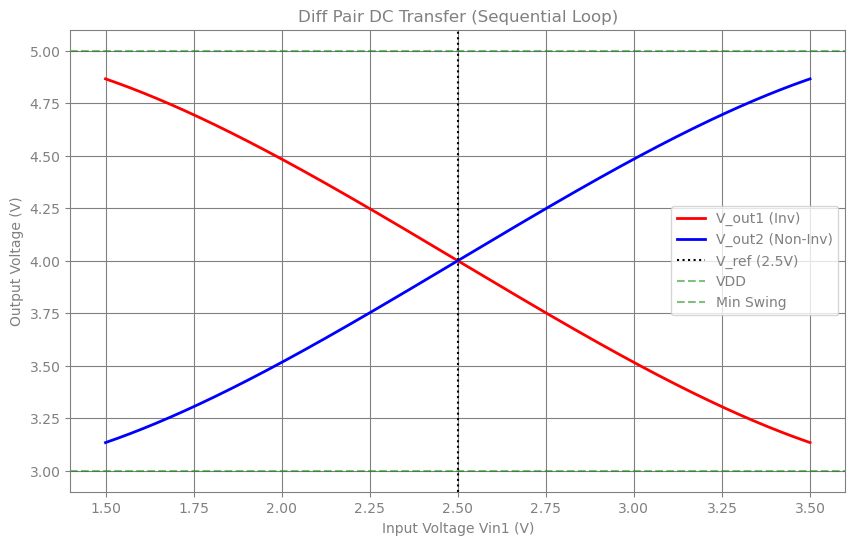
In this section, we analyze the MOS Differential Pair, the fundamental input stage of operational amplifiers and logic gates. The circuit consists of two matched NMOS transistors (\(M_1, M_2\)) sharing a common "tail" current source (\(I_{SS}\)).We will perform a DC Transfer Analysis, sweeping the input voltage \(V_{in1}\) from \(1.5V\) to \(3.5V\) while holding \(V_{in2}\) constant at \(2.5V\). This simulation reveals how the tail current steers between the two branches, creating the characteristic sigmoidal differential output.
Simulating a sweep in JAX requires a different mindset than standard Python loops:
-
Immutability: JAX arrays and circuit objects are immutable. We cannot simply do circuit.R1.value = 10. Instead, we define a functional update_param_value helper that returns a new circuit definition with the modified parameter.
-
Sequential Continuation (jax.lax.scan): Unlike a Monte Carlo simulation where every run is independent (perfect for vmap), a DC sweep works best when sequential. By using
jax.lax.scan, we feed the solution of the previous voltage step (y_prev) as the initial guess for the current step. This "homotopy" or continuation method drastically improves convergence stability for non-linear components like MOSFETs. -
Compilation: The entire sweep loop is compiled into a single XLA kernel, executing thousands of voltage steps in milliseconds.
import time

import jax
import jax.numpy as jnp
import matplotlib.pyplot as plt

from circulax import compile_circuit
from circulax.components.electronic import NMOS, CurrentSource, Resistor, VoltageSource

jax.config.update("jax_enable_x64", True)
net_dict = {
    "instances": {
        "GND": {"component": "ground"},
        "VDD": {"component": "source_dc", "settings": {"V": 5.0}},
        "Iss": {"component": "current_src", "settings": {"I": 1e-3}},
        "RD1": {"component": "resistor", "settings": {"R": 2000}},
        "RD2": {"component": "resistor", "settings": {"R": 2000}},
        "M1": {"component": "nmos", "settings": {"W": 50e-6, "L": 1e-6}},
        "M2": {"component": "nmos", "settings": {"W": 50e-6, "L": 1e-6}},
        "Vin1": {"component": "source_dc", "settings": {"V": 1.5}},
        "Vin2": {"component": "source_dc", "settings": {"V": 2.5}},
    },
    "connections": {
        "GND,p1": ("VDD,p2", "Vin1,p2", "Vin2,p2", "Iss,p2"),
        "Iss,p1": ("M1,s", "M2,s"),
        "M1,d": "RD1,p2",
        "M2,d": "RD2,p2",
        "RD1,p1": "VDD,p1",
        "RD2,p1": "VDD,p1",
        "Vin1,p1": "M1,g",
        "Vin2,p1": "M2,g",
    },
    "ports": {"out1": "RD1,p2", "out2": "RD2,p2"},
}

models_map = {
    "nmos": NMOS,
    "resistor": Resistor,
    "source_dc": VoltageSource,
    "current_src": CurrentSource,
    "ground": lambda: 0,
}

print("1. Compiling...")
circuit = compile_circuit(net_dict, models_map)


@jax.jit
def scan_step(y_prev, v_in_val):
    y_sol = circuit.dc(params={"Vin1.V": v_in_val}, y_guess=y_prev)
    return y_sol, y_sol


sweep_voltages = jnp.linspace(1.5, 3.5, 1000)

print(f"2. Running Sweep ({len(sweep_voltages)} points)...")
print("Sweeping DC Operating Point (with Continuation)...")
start_time = time.time()

y_current = jnp.zeros(circuit.sys_size)
# Using JAX scan, the previous solution is used as a guess for the sequential root solve
final_y, solutions = jax.lax.scan(scan_step, y_current, sweep_voltages)

total = time.time() - start_time
print(f"Simulation Time: {total:.3f}s")

v_out1 = circuit.port(solutions, "out1")
v_out2 = circuit.port(solutions, "out2")

plt.figure(figsize=(10, 6))
plt.plot(sweep_voltages, v_out1, "r-", linewidth=2, label="V_out1 (Inv)")
plt.plot(sweep_voltages, v_out2, "b-", linewidth=2, label="V_out2 (Non-Inv)")

plt.axvline(2.5, color="k", linestyle=":", label="V_ref (2.5V)")
plt.axhline(5.0, color="green", linestyle="--", alpha=0.5, label="VDD")
plt.axhline(5.0 - (1e-3 * 2000), color="green", linestyle="--", alpha=0.5, label="Min Swing")

plt.title("Diff Pair DC Transfer (Sequential Loop)")
plt.xlabel("Input Voltage Vin1 (V)")
plt.ylabel("Output Voltage (V)")
plt.legend()
plt.grid(True)
plt.show()
1. Compiling...


2. Running Sweep (1000 points)...
Sweeping DC Operating Point (with Continuation)...


Simulation Time: 0.466s