Silicon Ring Modulator: Electro-Optic Simulation¤
This notebook simulates the transient optical response of a ring resonator modulator using Temporal Coupled-Mode Theory (t-CMT). An optical pulse is launched into a bus waveguide coupled to the ring. We observe how the ring energy \(a(t)\) builds up and decays, and how this shapes the transmitted field.
This notebook covers four progressively more complex analyses:
- Part 1 Optical impulse response: Step-on/off pulse excites the ring, revealing the photon lifetime \(\tau\).
- Part 2 Small-signal EO bandwidth (time-domain sweep): AC voltage drives a PN junction; transient simulation extracts the EO 3-dB bandwidth.
- Part 3 EO bandwidth via Harmonic Balance: Same bandwidth measurement using
jax.vmapover frequency in a single JIT call. - Part 4 Large-signal NRZ eye diagram: 128-bit PRBS pattern at 56 GBaud reveals ISI from photon-lifetime memory.
- Part 5 \(V_\mathrm{bias}\) sweep via
jax.vmap: Four eye diagrams at different bias voltages, computed in a single vmapped transient call.
t-CMT equations¤
The complex ring energy \(a(t)\) (with \(|a|^2\) in units of energy) evolves as:
where \(\Delta\omega = 2\pi(f_{\rm op} - f_r) + V_{\rm wr}\,V\) is the laser\u2013resonance detuning, and \(1/\tau = 1/\tau_e + 1/\tau_l\) combines the coupling (\(\tau_e\)) and loss (\(\tau_l\)) photon lifetimes. The transmitted field is
Mapping to the circulax DAE (\(F + dQ/dt = 0\))¤
The RingModulator component below carries two internal states:
| State | \(F\)-term (residual) | \(Q\)-term (storage) | Role |
|---|---|---|---|
a | \(j\sqrt{2/\tau_e}\,V_{p1} - j\Delta\omega\,a + a/\tau\) | \(a\) | Ring energy ODE |
i_out | \(V_{p2}-(V_{p1}-j\sqrt{2/\tau_e}\,a)\) | -- | Output field constraint |
Port p1 (input) contributes zero current \u2014 the ring is transparent at the input (S11 = 0), so the source drives the input field directly. Port p2 (output) is driven by the auxiliary state i_out, which enforces the output field relation algebraically.
The ring energy can be recovered as a post-processing step directly from the port voltages: \(a = -j\,(E_i - E_o)/\sqrt{2/\tau_e}\).
References: Absil et al., OE 2000; Choi et al., OE 2015
import diffrax
import jax
import jax.numpy as jnp
import matplotlib.pyplot as plt
import numpy as np

from circulax import compile_circuit
from circulax.components.base_component import PhysicsReturn, Signals, States, component, source
from circulax.components.electronic import Resistor

jax.config.update("jax_enable_x64", True)
Component definitions¤
@source(ports=("p1", "p2"), states=("i_src",))
def OpticalSourcePulseOnOff(
    signals: Signals,
    s: States,
    t: float,
    power: float = 1.0,
    phase: float = 0.0,
    t_on: float = 50e-12,
    t_off: float = 150e-12,
    rise: float = 5e-12,
) -> PhysicsReturn:
    """CW optical source with a smooth rectangular pulse envelope.

    Two sigmoid ramps (one up, one down) define the on/off transitions.
    The rise-time constant ``rise`` should be chosen small relative to the
    photon lifetime to approximate a sharp turn-on/off.

    Args:
        signals: Field amplitudes at positive (``p1``) and negative (``p2``) ports.
        s: Source current state variable ``i_src``.
        t: Simulation time.
        power: Peak optical power in watts. Defaults to ``1.0``.
        phase: Output field phase in radians. Defaults to ``0.0``.
        t_on: Turn-on time in seconds. Defaults to ``50e-12``.
        t_off: Turn-off time in seconds. Defaults to ``150e-12``.
        rise: Sigmoid rise/fall time constant. Defaults to ``5e-12``.

    """
    sigmoid_on = jax.nn.sigmoid((t - t_on) / rise)
    sigmoid_off = jax.nn.sigmoid((t - t_off) / rise)
    amp = jnp.sqrt(power) * jnp.exp(1j * phase) * (sigmoid_on - sigmoid_off)
    constraint = (signals.p1 - signals.p2) - amp
    return {"p1": s.i_src, "p2": -s.i_src, "i_src": constraint}, {}


@component(ports=("p1", "p2"), states=("a", "i_out"))
def RingModulator(
    signals: Signals,
    s: States,
    ng: float = 3.8,
    L: float = 3.14159265e-5,
    gamma: float = 0.976,
    alpha0: float = 0.969,
    alpha1: float = 0.0,
    voltage: float = 0.0,
    f_operating: float = 2.2904e14,
    f_resonance: float = 2.2901e14,
    v_to_wr: float = 0.0,
) -> PhysicsReturn:
    """Optical ring modulator via Temporal Coupled-Mode Theory (t-CMT).

    Tracks the complex ring energy amplitude ``a(t)`` as an internal state and
    enforces the output field relation ``E_o = E_i - j sqrt(2/tau_e) a`` via an
    algebraic constraint state ``i_out``.

    The ring energy ODE is expressed in the circulax DAE form F + dQ/dt = 0:

    - F["a"] = -(da/dt RHS) = j sqrt(2/tau_e) V_p1 - j Delta_omega a + a/tau
    - Q["a"] = a

    Gives: da/dt = -j sqrt(2/tau_e) E_i + j Delta_omega a - a/tau.

    Port ``p1`` contributes zero current (S11 = 0 approximation).
    Port ``p2`` is driven by ``i_out`` which enforces the output field.

    Args:
        signals: Complex field amplitudes at input (``p1``) and output (``p2``).
        s: Internal states: ``a`` (complex ring energy) and ``i_out`` (output
            constraint current).
        ng: Group refractive index. Defaults to ``3.8``.
        L: Ring circumference in metres. Defaults to ``2*pi*5e-6``.
        gamma: Through-coupling amplitude coefficient. Defaults to ``0.976``.
        alpha0: Voltage-independent round-trip amplitude. Defaults to ``0.969``.
        alpha1: Linear voltage coefficient of round-trip amplitude (1/V).
            Defaults to ``0.0``.
        voltage: Applied DC bias voltage. Defaults to ``0.0``.
        f_operating: Laser frequency in Hz. Defaults to ``2.2904e14``.
        f_resonance: Ring resonance frequency in Hz. Defaults to ``2.2901e14``.
        v_to_wr: Electro-optic coefficient mapping voltage to resonance shift
            in rad/s/V. Defaults to ``0.0``.

    """
    c = 2.998e8  # speed of light, m/s

    # Photon lifetimes
    tau_e = 2.0 * ng * L / ((1.0 - gamma**2) * c)
    alpha_v = alpha0 + alpha1 * voltage
    tau_l = 2.0 * ng * L / ((1.0 - alpha_v**2) * c)
    tau = 1.0 / (1.0 / tau_e + 1.0 / tau_l)

    coupling = jnp.sqrt(2.0 / tau_e)

    # Laser-resonance detuning (+ EO shift)
    delta_omega = 2.0 * jnp.pi * (f_operating - f_resonance) + v_to_wr * voltage

    # Ring energy ODE RHS: da/dt = -j*coupling*E_i + j*delta_omega*a - a/tau
    rhs_a = -1j * coupling * signals.p1 + 1j * delta_omega * s.a - s.a / tau

    # Output field from the ring: E_o = E_i - j*coupling*a
    E_o_expected = signals.p1 - 1j * coupling * s.a

    f = {
        "p1": 0.0 + 0.0j,  # ring is transparent at input (S11=0)
        "p2": s.i_out,
        "i_out": signals.p2 - E_o_expected,  # enforce E_o = E_i - j*coupling*a
        "a": -rhs_a,  # ring energy ODE (negated RHS)
    }
    q = {"a": s.a}
    return f, q
Pattern: separating round-trip physics from CMT evaluation with .setup¤
For components whose CMT parameters are derived from physical device parameters (coupling coefficient κ, effective index n_eff, loss α, length L), the @<Component>.setup decorator cleanly separates the round-trip model from the CMT evaluation loop. The setup runs inside the JAX trace so gradients flow through it correctly — e.g. jax.grad(loss, kappa) traverses the sqrt(1 - κ²) inside .setup.
@component(ports=("in_", "thru"))
def RingMod(signals, s, init, kappa=0.3, neff=2.4, alpha=1e-3, L=..., V_pi=2.0, V=0.0):
    # init["a"], init["t"], init["phi"] were computed by the round-trip model below
    phi = init["phi"] * (1.0 + V / V_pi)
    H = (init["t"] - init["a"] * jnp.exp(1j * phi)) / (1 - init["t"] * init["a"] * jnp.exp(1j * phi))
    ...

@RingMod.setup
def _round_trip(kappa=0.3, neff=2.4, alpha=1e-3, L=...):
    """Derives a, t, phi₀ from physical device params."""
    return {
        "a":   jnp.exp(-alpha * L / 2.0),   # round-trip amplitude
        "t":   jnp.sqrt(1.0 - kappa**2),    # through-coupling
        "phi": 2.0 * jnp.pi * neff * L,     # round-trip phase at resonance
    }
The full runnable example and gradient tests are in tests/test_setup_decorator.py.
# ── Round-trip → CMT RingMod: demonstrating @Component.setup ──────────────────
# This cell is illustrative. Parts 1–5 below use RingModulator/RingModulatorEO
# which fold the round-trip computation inline for conciseness.


@component(ports=("in_", "thru"))
def RingModSetup(
    signals: Signals,
    s: States,
    init,
    kappa: float = 0.3,
    neff: float = 2.4,
    alpha: float = 1e-3,
    L: float = float(2 * jnp.pi * 5e-6),
    V_pi: float = 2.0,
    V: float = 0.0,
) -> PhysicsReturn:
    """All-pass ring response via CMT, using init coefficients from .setup."""
    phi = init["phi"] * (1.0 + V / V_pi)
    ejphi = jnp.exp(1j * phi)
    H = (init["t"] - init["a"] * ejphi) / (1.0 - init["t"] * init["a"] * ejphi)
    absorbed = (1.0 - jnp.abs(H) ** 2) * signals.in_
    return {"in_": absorbed, "thru": signals.thru - H * signals.in_}, {}


@RingModSetup.setup
def _round_trip(
    kappa: float = 0.3,
    neff: float = 2.4,
    alpha: float = 1e-3,
    L: float = float(2 * jnp.pi * 5e-6),
) -> dict:
    """Round-trip model: derive CMT coefficients from physical device parameters."""
    return {
        "a": jnp.exp(-alpha * L / 2.0),   # round-trip amplitude (loss)
        "t": jnp.sqrt(1.0 - kappa**2),    # through-coupling amplitude
        "phi": 2.0 * jnp.pi * neff * L,   # round-trip phase at reference wavelength
    }


# Functional check: evaluate the component (a lossless all-pass ring has |H|=1 for any phi)
rm_demo = RingModSetup(kappa=0.3, neff=2.4, alpha=1e-3)
f_demo, _ = rm_demo(in_=1.0 + 0j, thru=0.0 + 0j)
print(f"E_thru = {complex(f_demo['thru']):.4f}   |H| = {float(jnp.abs(f_demo['thru'])):.6f}")

# Gradient of the through-field phase w.r.t. kappa flows through the .setup body:
# kappa → t = sqrt(1-kappa^2) → H  (analytic dφ/dκ = -κ/t)
grad_kappa = jax.grad(
    lambda k: jnp.angle(RingModSetup(kappa=k)(in_=1.0 + 0j, thru=0.0 + 0j)[0]["thru"])
)(0.3)
print(f"d∠(E_thru)/dκ at κ=0.3 = {float(grad_kappa):.6f} rad  (non-zero gradient through .setup)")
E_thru = 0.9998+0.0201j   |H| = 0.999999


d∠(E_thru)/dκ at κ=0.3 = -0.140432 rad  (non-zero gradient through .setup)
Simulation parameters¤
Parameters are taken from the reference silicon photonics ring modulator in Choi et al., OE 2015.
c = 2.998e8  # m/s

# Ring geometry and coupling
ng = 3.8
radius_um = 5.0  # ring radius, μm
L_ring = float(2.0 * np.pi * radius_um * 1e-6)  # circumference, m
gamma = 0.976  # through-coupling amplitude
alpha0 = 0.969  # round-trip amplitude (unbiased)

# Operating wavelength – 0.30 nm blue-detuned from resonance.
# This gives Δω·τ ≈ 2.4, producing ~1–2 visible ringing cycles during the
# ~3τ transient when the source turns on with a sharp (1 ps) rise time.
wavelength_res_nm = 1310.0
detuning_nm = 0.30
wavelength_op_nm = wavelength_res_nm - detuning_nm

f_resonance = c / (wavelength_res_nm * 1e-9)
f_operating = c / (wavelength_op_nm * 1e-9)

# Derived photon lifetimes
tau_e = 2.0 * ng * L_ring / ((1.0 - gamma**2) * c)
tau_l = 2.0 * ng * L_ring / ((1.0 - alpha0**2) * c)
tau = 1.0 / (1.0 / tau_e + 1.0 / tau_l)
coupling = np.sqrt(2.0 / tau_e)

# Ringing oscillation period: beats between laser and ring resonance
delta_f = f_operating - f_resonance
T_osc = 1.0 / delta_f  # period of output power oscillation during transient

# Steady-state transmission (analytic)
A = 2.0 * tau / tau_e
x = 2.0 * np.pi * delta_f * tau  # normalised detuning Δω·τ
T_ss = np.sqrt(((1 - A) ** 2 + x**2) / (1 + x**2))

print(f"Ring circumference : L = {L_ring * 1e6:.2f} μm  (R = {radius_um} μm)")
print(f"Coupling lifetime  : τ_e = {tau_e * 1e12:.1f} ps")
print(f"Loss lifetime      : τ_l = {tau_l * 1e12:.1f} ps")
print(f"Photon lifetime    : τ   = {tau * 1e12:.2f} ps")
print(f"Laser detuning     : Δf  = {delta_f / 1e9:.1f} GHz  ({detuning_nm} nm)  →  Δω·τ = {x:.2f}")
print(f"Ringing period     : T_osc = {T_osc * 1e12:.1f} ps  (~{3 * tau / T_osc:.1f} cycles during rise)")
print(f"Steady-state |T|   : {T_ss:.3f}  ({20 * np.log10(T_ss):.1f} dB)")
Ring circumference : L = 31.42 μm  (R = 5.0 μm)
Coupling lifetime  : τ_e = 16.8 ps
Loss lifetime      : τ_l = 13.0 ps
Photon lifetime    : τ   = 7.34 ps
Laser detuning     : Δf  = 52.4 GHz  (0.3 nm)  →  Δω·τ = 2.42
Ringing period     : T_osc = 19.1 ps  (~1.2 cycles during rise)
Steady-state |T|   : 0.925  (-0.7 dB)
Netlist and compilation¤
rise_time = 1e-12  # 1 ps rise/fall — sharp enough to excite ring ringing clearly

models_map = {
    "ground": lambda: 0,
    "source_pulse_onoff": OpticalSourcePulseOnOff,
    "ring_modulator": RingModulator,
    "resistor": Resistor,
}

net_dict = {
    "instances": {
        "GND": {"component": "ground"},
        "Src": {
            "component": "source_pulse_onoff",
            "settings": {
                "power": 1.0,
                "t_on": 50e-12,
                "t_off": 150e-12,
                "rise": rise_time,
            },
        },
        "Ring": {
            "component": "ring_modulator",
            "settings": {
                "ng": ng,
                "L": L_ring,
                "gamma": gamma,
                "alpha0": alpha0,
                "f_operating": float(f_operating),
                "f_resonance": float(f_resonance),
            },
        },
        "Load": {"component": "resistor", "settings": {"R": 1.0}},
    },
    "connections": {
        "GND,p1": ("Src,p2", "Load,p2"),  # common ground
        "Src,p1": "Ring,p1",  # source output → ring input
        "Ring,p2": "Load,p1",  # ring output → load
    },
    "ports": {"in": "Src,p1", "out": "Ring,p2"},
}

print("Compiling netlist...")
circuit = compile_circuit(net_dict, models_map, is_complex=True)
print(f"System size: {circuit.sys_size} real nodes")
Compiling netlist...


System size: 6 real nodes
DC operating point¤
At \(t = 0\) the source is off, so the DC operating point is trivially zero.
Transient simulation¤
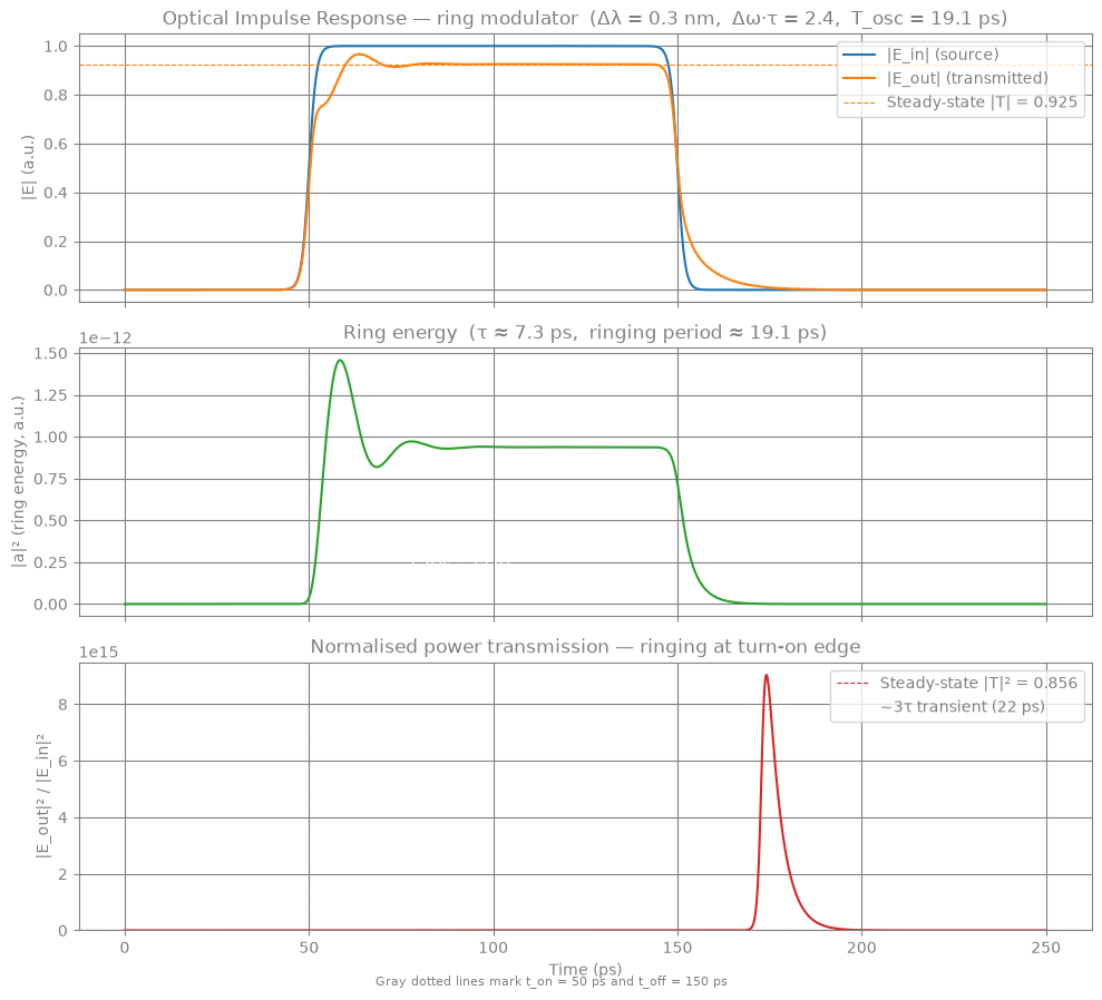
The simulation runs for 250 ps, long enough to see both the ring energy buildup (\(\sim 3\tau \approx 22\,\text{ps}\) to reach 95\%) and the decay after the optical pulse is switched off.
Convergence note: dtmax in the step-size controller¤
With a 1 ps rise time, the adaptive PID step-size controller will eventually grow the step to \(\gg 1\,\text{ps}\). When a single step spans the entire transition, the linear predictor lands far from the true solution, the Newton residual becomes large, and the built-in damping (DAMPING_FACTOR = 0.5) shrinks each Newton update to \(\lesssim 0.5 / \Delta_{\rm max}\).
The fix is dtmax = rise_time / 2 in PIDController, which prevents any single step from spanning the source transition. This keeps the predictor accurate and Newton convergence fast.
t_end = 250e-12  # 250 ps
num_points = 2500

controller = diffrax.PIDController(
    rtol=1e-4,
    atol=1e-6,
    dtmax=rise_time / 2,  # keep steps within the source rise time
)

print("Running transient simulation...")
sol = circuit.transient(
    t0=0.0,
    t1=t_end,
    dt0=1e-13,
    y0=y0,
    saveat=diffrax.SaveAt(ts=jnp.linspace(0.0, t_end, num_points)),
    max_steps=500000,
    throw=False,
    stepsize_controller=controller,
)

if sol.result == diffrax.RESULTS.successful:
    print("Simulation successful")
else:
    print(f"Simulation ended with: {sol.result}")
Running transient simulation...


Simulation successful
Results¤
The input and output fields are read through named top-level ports. The ring energy Ring,a is an internal state, so it is inspected by its component-state name.
ts_ps = sol.ts * 1e12

E_in = circuit.port(sol.ys, "in")
E_out = circuit.port(sol.ys, "out")
a_val = circuit.port(sol.ys, "Ring,a")

P_in = jnp.abs(E_in) ** 2
P_out = jnp.abs(E_out) ** 2
eps = 1e-20

fig, axes = plt.subplots(3, 1, figsize=(10, 9), sharex=True)

t_on_ps = 50.0
T_osc_ps = T_osc * 1e12

axes[0].plot(ts_ps, jnp.abs(E_in), color="tab:blue", linewidth=1.5, label="|E_in| (source)")
axes[0].plot(ts_ps, jnp.abs(E_out), color="tab:orange", linewidth=1.5, label="|E_out| (transmitted)")
axes[0].axhline(T_ss, color="tab:orange", linestyle="--", linewidth=0.8, label=f"Steady-state |T| = {T_ss:.3f}")
axes[0].set_ylabel("|E| (a.u.)")
axes[0].set_title(
    f"Optical Impulse Response — ring modulator  (Δλ = {detuning_nm} nm,  Δω·τ = {x:.1f},  T_osc = {T_osc_ps:.1f} ps)"
)
axes[0].legend(loc="upper right")

axes[1].plot(ts_ps, jnp.abs(a_val) ** 2, color="tab:green", linewidth=1.5)
axes[1].set_ylabel("|a|² (ring energy, a.u.)")
axes[1].set_title(f"Ring energy  (τ ≈ {tau * 1e12:.1f} ps,  ringing period ≈ {T_osc_ps:.1f} ps)")

a2_ss = (2.0 / tau_e) * tau**2 / (1 + x**2)
axes[1].annotate(
    f"T_osc ≈ {T_osc_ps:.0f} ps",
    xy=(t_on_ps + T_osc_ps, a2_ss * 0.5),
    xytext=(t_on_ps + T_osc_ps + 8, a2_ss * 0.25),
    arrowprops=dict(arrowstyle="->", color="white"),
    color="white",
    fontsize=9,
)

P_out_norm = P_out / (P_in + eps)
axes[2].plot(ts_ps, P_out_norm, color="tab:red", linewidth=1.5)
axes[2].axhline(T_ss**2, color="tab:red", linestyle="--", linewidth=0.8, label=f"Steady-state |T|² = {T_ss**2:.3f}")
axes[2].axvspan(t_on_ps, t_on_ps + 3 * tau * 1e12, alpha=0.08, color="white", label=f"~3τ transient ({3 * tau * 1e12:.0f} ps)")
axes[2].set_ylabel("|E_out|² / |E_in|²")
axes[2].set_xlabel("Time (ps)")
axes[2].set_title("Normalised power transmission — ringing at turn-on edge")
axes[2].legend(loc="upper right")
axes[2].set_ylim(bottom=0)

for ax in axes:
    ax.axvline(50, color="gray", linestyle=":", linewidth=0.8, alpha=0.6)
    ax.axvline(150, color="gray", linestyle=":", linewidth=0.8, alpha=0.6)

fig.text(0.5, 0.01, "Gray dotted lines mark t_on = 50 ps and t_off = 150 ps", ha="center", color="gray", fontsize=8)

fig.tight_layout()
plt.show()

mid = num_points // 2
print(f"Simulated steady-state |T|: {float(jnp.abs(E_out[mid]) / (jnp.abs(E_in[mid]) + eps)):.3f}")
print(f"Analytic  steady-state |T|: {T_ss:.3f}")
Simulated steady-state |T|: 0.925
Analytic  steady-state |T|: 0.925
Small-signal electro-optic bandwidth¤
Note — time-domain is overkill here. A proper small-signal AC analysis or a Harmonic Balance (HB) solver would extract the EO frequency response in a single solve at each frequency, without integrating through many AC periods. circulax already has a Harmonic Balance solver and small-signal AC analysis is a planned feature. The purpose of this section is to verify that the time-domain DAE equations are equivalent to the analytic transfer function — i.e. the equations are correct — not to advocate transient simulation as the right tool for bandwidth characterisation in production.
A small sinusoidal voltage is applied to the ring modulator through an RC equivalent circuit that models a reverse-biased PN junction:
- R_s — series resistance (contact + waveguide)
- C_j — depletion capacitance (junction)
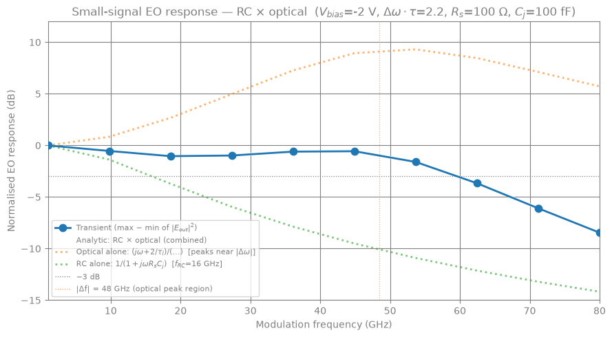
The combined small-signal EO response is limited by two first-order poles:
where \(f_{\rm RC} = 1/(2\pi R_s C_j)\) and \(f_{\rm opt} = 1/(2\pi\tau)\).
Simulation strategy: the DC operating point (optical CW + DC bias \(V_{\rm bias}\)) is found first and used as the initial condition at \(t = 0\). A small AC swing \(V_{\rm ac}\sin(2\pi f t)\) is then enabled at \(t = 10\,\text{ps}\). For each modulation frequency the output power amplitude (max \(-\) min of \(|E_{\rm out}|^2\)) is extracted from the last half of the simulation and normalised to the low-frequency value.
from circulax.components.electronic import Capacitor


@source(ports=("p1", "p2"), states=("i_src",))
def OpticalSourceStep(
    signals: Signals,
    s: States,
    t: float,
    power: float = 1.0,
    phase: float = 0.0,
) -> PhysicsReturn:
    """Constant-amplitude optical CW source (always on, no time dependence)."""
    amp = jnp.sqrt(power) * jnp.exp(1j * phase)
    constraint = (signals.p1 - signals.p2) - amp
    return {"p1": s.i_src, "p2": -s.i_src, "i_src": constraint}, {}


@source(ports=("p1", "p2"), states=("i_src",))
def BiasedACSource(
    signals: Signals,
    s: States,
    t: float,
    V_bias: float = -2.0,
    V_ac: float = 0.1,
    freq: float = 1e9,
    t_ac_start: float = 10e-12,
    rise_ac: float = 1e-12,
) -> PhysicsReturn:
    """DC-biased sinusoidal voltage source.

    Outputs V_bias (always present) plus V_ac * sin(2π * freq * t), with the
    AC component enabled smoothly at t_ac_start.  At t=0 the AC term is
    negligibly small (sigmoid(-10) ≈ 0), so solve_dc finds the correct DC
    operating point with only V_bias present.
    """
    v_ac = V_ac * jnp.sin(2.0 * jnp.pi * freq * t)
    ac_enable = jax.nn.sigmoid((t - t_ac_start) / rise_ac)
    v_total = V_bias + v_ac * ac_enable
    constraint = (signals.p1 - signals.p2) - v_total
    return {"p1": s.i_src, "p2": -s.i_src, "i_src": constraint}, {}


@component(ports=("p1", "p2", "v_e"), states=("a", "i_out"))
def RingModulatorEO(
    signals: Signals,
    s: States,
    ng: float = 3.8,
    L: float = 3.14159265e-5,
    gamma: float = 0.976,
    alpha0: float = 0.969,
    alpha1: float = 0.0,
    f_operating: float = 2.2904e14,
    f_resonance: float = 2.2901e14,
    v_to_wr: float = 0.0,
) -> PhysicsReturn:
    """Ring modulator with an external electrical voltage port ``v_e``.

    The voltage at port ``v_e`` modulates the ring resonance frequency via
    ``v_to_wr`` (rad/s/V).  The port is high-impedance: it draws no current
    (``F["v_e"] = 0``), so any driver circuit sees an open circuit.

    The physics is otherwise identical to :func:`RingModulator`, but ``voltage``
    is read from the external port rather than being a fixed parameter.
    """
    c = 2.998e8
    voltage = jnp.real(signals.v_e)  # electrical port — real part only

    tau_e = 2.0 * ng * L / ((1.0 - gamma**2) * c)
    alpha_v = alpha0 + alpha1 * voltage
    tau_l = 2.0 * ng * L / ((1.0 - alpha_v**2) * c)
    tau = 1.0 / (1.0 / tau_e + 1.0 / tau_l)
    coupling = jnp.sqrt(2.0 / tau_e)

    delta_omega = 2.0 * jnp.pi * (f_operating - f_resonance) + v_to_wr * voltage

    rhs_a = -1j * coupling * signals.p1 + 1j * delta_omega * s.a - s.a / tau
    E_o_expected = signals.p1 - 1j * coupling * s.a

    f = {
        "p1": 0.0 + 0.0j,
        "p2": s.i_out,
        "v_e": 0.0 + 0.0j,  # high-impedance electrical port
        "i_out": signals.p2 - E_o_expected,
        "a": -rhs_a,
    }
    q = {"a": s.a}
    return f, q
# ── Electrical RC parameters ──────────────────────────────────────────────
V_bias = -2.0  # V   — DC reverse bias (negative = reverse-biased PN junction)
V_ac = 0.2  # V   — small-signal swing (<<1, so response is linear)
R_s = 100.0  # Ω   — series resistance (contact + waveguide)
C_j = 100e-15  # F   — junction depletion capacitance
v_to_wr = 2.0 * np.pi * 2e9  # rad/s/V — EO coefficient (2 GHz/V resonance shift)
t_ac_start = 10e-12  # s   — delay before AC is enabled

f_RC = 1.0 / (2.0 * np.pi * R_s * C_j)  # electrical 3-dB bandwidth
f_opt_bw = 1.0 / (2.0 * np.pi * tau)  # optical photon-lifetime bandwidth

print(f"Electrical RC bandwidth : f_RC  = {f_RC / 1e9:.1f} GHz")
print(f"Optical photon-lifetime : f_opt = {f_opt_bw / 1e9:.1f} GHz")
print(f"EO coefficient          : dω/dV = {v_to_wr / (2e9 * np.pi):.1f} × 2π GHz/V")

# ── Models map ────────────────────────────────────────────────────────
models_map_ss = {
    "ground": lambda: 0,
    "optical_cw": OpticalSourceStep,
    "biased_ac": BiasedACSource,
    "ring_eo": RingModulatorEO,
    "resistor": Resistor,
    "capacitor": Capacitor,
}

# ── Netlist ───────────────────────────────────────────────────────────────────
# Topology:
#   OptSrc → Ring (optical path)
#   Vsrc → Rs → node_ve → Cj → GND  (electrical RC network)
#   Ring,v_e = node_ve  (high-impedance; ring reads voltage, draws no current)
net_dict_ss = {
    "instances": {
        "GND": {"component": "ground"},
        "OptSrc": {"component": "optical_cw", "settings": {"power": 1.0}},
        "Ring": {
            "component": "ring_eo",
            "settings": {
                "ng": ng,
                "L": L_ring,
                "gamma": gamma,
                "alpha0": alpha0,
                "f_operating": float(f_operating),
                "f_resonance": float(f_resonance),
                "v_to_wr": v_to_wr,
            },
        },
        "Load": {"component": "resistor", "settings": {"R": 1.0}},
        "Vsrc": {
            "component": "biased_ac",
            "settings": {
                "V_bias": V_bias,
                "V_ac": V_ac,
                "freq": 1e9,
                "t_ac_start": t_ac_start,
            },
        },
        "Rs": {"component": "resistor", "settings": {"R": R_s}},
        "Cj": {"component": "capacitor", "settings": {"C": C_j}},
    },
    "connections": {
        "GND,p1": ("OptSrc,p2", "Load,p2", "Vsrc,p2", "Cj,p2"),
        "OptSrc,p1": "Ring,p1",
        "Ring,p2": "Load,p1",
        "Vsrc,p1": "Rs,p1",
        "Rs,p2": ("Cj,p1", "Ring,v_e"),  # node_ve: RC junction & ring voltage port
    },
    "ports": {"in": "Ring,p1", "out": "Ring,p2", "ve": "Ring,v_e"},
}

print("\nCompiling small-signal netlist...")
circuit_ss = compile_circuit(net_dict_ss, models_map_ss, is_complex=True)
y0_ss = circuit_ss.dc()

# Report DC state
V_ve_dc = float(jnp.real(circuit_ss.port(y0_ss, "ve")))
E_in_dc = circuit_ss.port(y0_ss, "in")
E_out_dc = circuit_ss.port(y0_ss, "out")
T_dc_sim = float(jnp.abs(E_out_dc) / (jnp.abs(E_in_dc) + 1e-20))

# Analytic DC transmission at the biased detuning
delta_omega_dc = 2.0 * np.pi * (f_operating - f_resonance) + v_to_wr * V_bias
x_dc = delta_omega_dc * tau
A_dc = 2.0 * tau / tau_e
T_dc_analytic = np.sqrt(((1 - A_dc) ** 2 + x_dc**2) / (1 + x_dc**2))

print(f"\nDC node_ve voltage : {V_ve_dc:.3f} V  (expected {V_bias:.1f} V)")
print(f"DC |T| simulated   : {T_dc_sim:.4f}")
print(f"DC |T| analytic    : {T_dc_analytic:.4f}")
print(f"DC Δω·τ            : {x_dc:.3f}")
Electrical RC bandwidth : f_RC  = 15.9 GHz
Optical photon-lifetime : f_opt = 21.7 GHz
EO coefficient          : dω/dV = 2.0 × 2π GHz/V

Compiling small-signal netlist...


DC node_ve voltage : -2.000 V  (expected -2.0 V)
DC |T| simulated   : 0.9142
DC |T| analytic    : 0.9142
DC Δω·τ            : 2.234
freqs_GHz = np.linspace(1.0, 80, 10)
N_periods = 10.0  # simulate this many AC periods per run
n_save = 500  # save this many points in the readout window
amplitudes = []  # will hold max(P_out) - min(P_out) per frequency

print(f"Running {len(freqs_GHz)}-point frequency sweep …")
for idx, f_ghz in enumerate(freqs_GHz):
    f_hz = f_ghz * 1e9

    t_sim = t_ac_start + N_periods / f_hz
    t_read = t_ac_start + (N_periods // 2) / f_hz
    ts_save = jnp.linspace(t_read, t_sim, n_save)

    dtmax = 1.0 / (20.0 * f_hz)  # ≥ 20 samples per AC period

    sol = circuit_ss.transient(
        t0=0.0,
        t1=t_sim,
        dt0=min(1e-12, dtmax),
        y0=y0_ss,
        saveat=diffrax.SaveAt(ts=ts_save),
        max_steps=2_000_000,
        throw=False,
        params={"Vsrc.freq": f_hz},
        stepsize_controller=diffrax.PIDController(rtol=1e-8, atol=1e-8, dtmax=dtmax),
    )

    if sol.result != diffrax.RESULTS.successful:
        print(f"  [{idx + 1:2d}/{len(freqs_GHz)}] {f_ghz:5.1f} GHz  WARNING: {sol.result}")

    P_out = jnp.abs(circuit_ss.port(sol.ys, "out")) ** 2
    P_norm = jnp.min(P_out[: int(-n_save / 2)])
    amplitudes.append(float(jnp.max(P_out[: int(-n_save / 2)]) - P_norm))

    if (idx + 1) % 2 == 0:
        print(f"  {idx + 1}/{len(freqs_GHz)} done")

print("Sweep complete.")
Running 10-point frequency sweep …


  2/10 done


  4/10 done


  6/10 done


  8/10 done


  10/10 done
Sweep complete.
omega_m = 2.0 * np.pi * freqs_GHz * 1e9  # rad/s

delta_omega_dc = 2.0 * np.pi * (float(f_operating) - float(f_resonance)) + v_to_wr * V_bias
inv_tau = 1.0 / tau
inv_tau_l = 1.0 / tau_l

# Electrical RC lowpass
H_RC = 1.0 / (1.0 + 1j * omega_m * R_s * C_j)

# Second-order optical transfer function
#   H_opt(jω) = (jω + 2/τ_l) / (Δω² + (1/τ)² − ω² + j(2/τ)ω)
denom_dc = delta_omega_dc**2 + inv_tau**2
H_opt = (1j * omega_m + 2.0 * inv_tau_l) / (-(omega_m**2) + 1j * 2.0 * inv_tau * omega_m + denom_dc)

H_total = H_RC * H_opt
H_mag = np.abs(H_total)
H_norm = H_mag / H_mag[0]
H_dB = 20.0 * np.log10(H_norm)

H_RC_dB = 20.0 * np.log10(np.abs(H_RC) / np.abs(H_RC[0]))
H_opt_dB = 20.0 * np.log10(np.abs(H_opt) / np.abs(H_opt[0]))

f_pole_GHz = np.sqrt(delta_omega_dc**2 + inv_tau**2) / (2.0 * np.pi * 1e9)

amps = np.array(amplitudes)
amps_norm = amps / (amps[0])
amps_dB = 20.0 * np.log10(amps_norm)

print(f"DC-biased detuning  Δf      : {delta_omega_dc / (2 * np.pi * 1e9):.1f} GHz  (Δω·τ = {delta_omega_dc * tau:.2f})")
print(f"Optical pole magnitude      : {f_pole_GHz:.1f} GHz")
print(f"Optical peak (no RC)        : {float(np.max(H_opt_dB)):.1f} dB  at {freqs_GHz[np.argmax(H_opt_dB)]:.1f} GHz")
print(f"Combined peak (RC + optical): {float(np.max(H_dB)):.1f} dB  at {freqs_GHz[np.argmax(H_dB)]:.1f} GHz")

fig, ax = plt.subplots(figsize=(9, 5))

ax.plot(freqs_GHz, amps_dB, "o-", ms=7.5, linewidth=2.0, zorder=3, label="Transient (max − min of $|E_{out}|^2$)")
ax.plot(freqs_GHz, H_dB, "w--", linewidth=3.0, label="Analytic: RC × optical (combined)")
ax.plot(
    freqs_GHz,
    H_opt_dB,
    ":",
    linewidth=2.0,
    alpha=0.6,
    label=r"Optical alone: $(j\omega\!+\!2/\tau_l)/(…)$  [peaks near $|\Delta\omega|$]",
)
ax.plot(
    freqs_GHz,
    H_RC_dB,
    ":",
    linewidth=2.0,
    alpha=0.6,
    label=f"RC alone: $1/(1+j\\omega R_s C_j)$  [$f_{{RC}}$={f_RC / 1e9:.0f} GHz]",
)

ax.axhline(-3.0, color="gray", linestyle=":", linewidth=0.9, label="−3 dB")
ax.axvline(
    abs(delta_omega_dc) / (2 * np.pi * 1e9),
    color="tab:orange",
    linestyle=":",
    linewidth=0.9,
    alpha=0.7,
    label=f"|Δf| = {abs(delta_omega_dc) / (2 * np.pi * 1e9):.0f} GHz (optical peak region)",
)

ax.set_xlabel("Modulation frequency (GHz)")
ax.set_ylabel("Normalised EO response (dB)")
ax.set_title(
    f"Small-signal EO response — RC × optical  "
    f"($V_{{bias}}$={V_bias:.0f} V, $\\Delta\\omega\\cdot\\tau$={delta_omega_dc * tau:.1f}, "
    f"$R_s$={R_s:.0f} Ω, $C_j$={C_j * 1e15:.0f} fF)"
)
ax.set_xlim(freqs_GHz[0], freqs_GHz[-1])
ax.set_ylim(-15.0, 12.0)
ax.legend(fontsize=8, loc="lower left")
fig.tight_layout()
plt.show()
DC-biased detuning  Δf      : 48.4 GHz  (Δω·τ = 2.23)
Optical pole magnitude      : 53.1 GHz
Optical peak (no RC)        : 9.3 dB  at 53.7 GHz
Combined peak (RC + optical): 0.0 dB  at 1.0 GHz
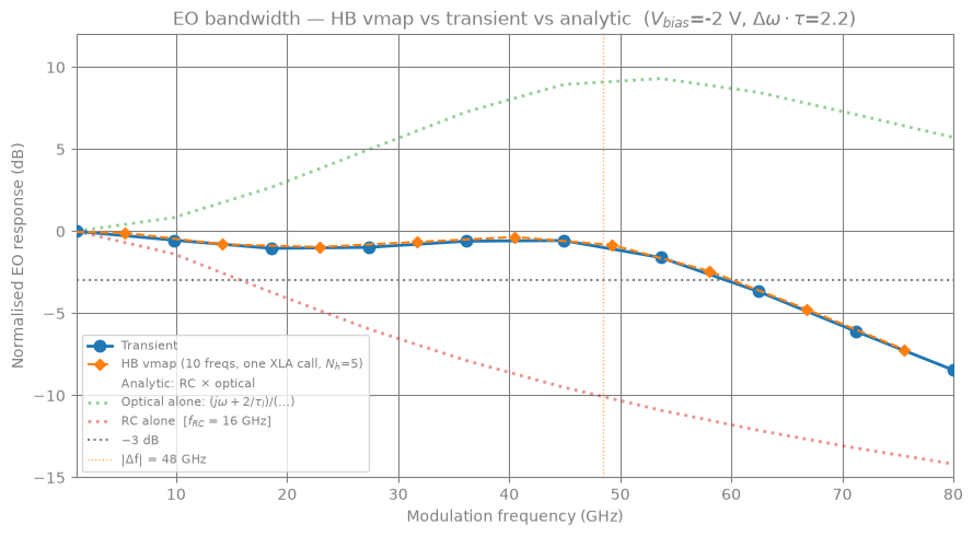
Part 3: EO Bandwidth via Harmonic Balance¤
The transient sweep above runs independent simulations — one per frequency. Harmonic Balance (HB) finds the periodic steady state directly, without time-stepping to steady state, and jax.vmap solves all frequencies in a single XLA compilation.
The modulation frequency \(f_m\) is the HB fundamental. With \(N_h = 5\) harmonics (\(K = 11\) time samples per period) the Newton loop converges in ~20 iterations independent of \(f_m\).
How the sweep works¤
def hb_sweep_point(freq):
    y_time, _ = circuit_hb.hb(
        freq=freq,
        harmonics=N_harm_hb,
        y0=y_dc_hb,
        params={"Vsrc.freq": freq},
    )
    E_out = circuit_hb.port(y_time, "out")
    return jnp.max(jnp.abs(E_out) ** 2) - jnp.min(jnp.abs(E_out) ** 2)

amps_hb = jax.jit(jax.vmap(hb_sweep_point))(sweep_freqs)
compile_circuit(..., is_complex=True) configures the photonic circuit; circuit.hb(...) handles the complex block representation internally.
@source(ports=("p1", "p2"), states=("i_src",))
def BiasedSinSource(
    signals: Signals,
    s: States,
    t: float,
    V_bias: float = -2.0,
    V_ac: float = 0.1,
    freq: float = 1e9,
) -> PhysicsReturn:
    """DC-biased sinusoidal source, exactly periodic at ``freq``.

    At t = 0: V = V_bias (no AC), giving the same DC operating point as
    :class:`BiasedACSource` with the AC component disabled.
    """
    v = V_bias + V_ac * jnp.sin(2.0 * jnp.pi * freq * t)
    return {"p1": s.i_src, "p2": -s.i_src, "i_src": (signals.p1 - signals.p2) - v}, {}


models_map_hb = {
    "ground": lambda: 0,
    "optical_cw": OpticalSourceStep,
    "biased_sin": BiasedSinSource,
    "ring_eo": RingModulatorEO,
    "resistor": Resistor,
    "capacitor": Capacitor,
}

net_dict_hb = {
    "instances": {
        "GND": {"component": "ground"},
        "OptSrc": {"component": "optical_cw", "settings": {"power": 1.0}},
        "Ring": {
            "component": "ring_eo",
            "settings": {
                "ng": ng,
                "L": L_ring,
                "gamma": gamma,
                "alpha0": alpha0,
                "f_operating": float(f_operating),
                "f_resonance": float(f_resonance),
                "v_to_wr": v_to_wr,
            },
        },
        "Load": {"component": "resistor", "settings": {"R": 1.0}},
        "Vsrc": {
            "component": "biased_sin",
            "settings": {
                "V_bias": V_bias,
                "V_ac": V_ac,
                "freq": 1e9,  # placeholder; updated per sweep point
            },
        },
        "Rs": {"component": "resistor", "settings": {"R": R_s}},
        "Cj": {"component": "capacitor", "settings": {"C": C_j}},
    },
    "connections": {
        "GND,p1": ("OptSrc,p2", "Load,p2", "Vsrc,p2", "Cj,p2"),
        "OptSrc,p1": "Ring,p1",
        "Ring,p2": "Load,p1",
        "Vsrc,p1": "Rs,p1",
        "Rs,p2": ("Cj,p1", "Ring,v_e"),
    },
    "ports": {"in": "Ring,p1", "out": "Ring,p2", "ve": "Ring,v_e"},
}

print("Compiling HB netlist...")
circuit_hb = compile_circuit(net_dict_hb, models_map_hb, is_complex=True)
y_dc_hb = circuit_hb.dc()

E_in_dc_hb = circuit_hb.port(y_dc_hb, "in")
E_out_dc_hb = circuit_hb.port(y_dc_hb, "out")
T_dc_hb = float(jnp.abs(E_out_dc_hb) / (jnp.abs(E_in_dc_hb) + 1e-20))
print(f"\nDC |T| (HB netlist) : {T_dc_hb:.4f}  (transient: {T_dc_sim:.4f})")
Compiling HB netlist...


DC |T| (HB netlist) : 0.9142  (transient: 0.9142)
N_harm_hb = 5  # 5 harmonics → K = 11 time samples per period
K_hb = 2 * N_harm_hb + 1
f_demo = 1e9  # 1 GHz single-point demo

y_time_demo, _ = circuit_hb.hb(
    freq=f_demo,
    harmonics=N_harm_hb,
    y0=y_dc_hb,
    params={"Vsrc.freq": f_demo},
)
print(f"HB converged at {f_demo / 1e9:.0f} GHz.  y_time shape: {y_time_demo.shape}")

T_period_demo = 1.0 / f_demo
t_hb_demo = np.linspace(0, T_period_demo * 1e9, K_hb, endpoint=False)  # ns

E_in_demo = circuit_hb.port(y_time_demo, "in")
E_out_demo = circuit_hb.port(y_time_demo, "out")
P_in_demo = jnp.abs(E_in_demo) ** 2
P_out_demo = jnp.abs(E_out_demo) ** 2

fig, ax = plt.subplots(figsize=(8, 3.5))
ax.plot(t_hb_demo, np.array(P_in_demo), "C0o-", ms=7, label=r"$|E_\mathrm{in}|^2$  (CW)")
ax.plot(t_hb_demo, np.array(P_out_demo), "C1s-", ms=7, label=r"$|E_\mathrm{out}|^2$  (modulated)")
ax.axhline(T_dc_hb**2, color="C1", ls="--", lw=0.8, label=f"DC $|T|^2 = {T_dc_hb**2:.3f}$")
ax.set_xlabel("Time (ns)")
ax.set_ylabel("Power (a.u.)")
ax.set_title(f"HB waveform at $f_m$ = {f_demo / 1e9:.0f} GHz  ($K$ = {K_hb} points, $N_h$ = {N_harm_hb})")
ax.legend()
plt.tight_layout()
plt.show()

amp_demo = float(jnp.max(P_out_demo) - jnp.min(P_out_demo))
print(f"P_out oscillation amplitude: {amp_demo:.4e} W  (peak-to-peak power modulation)")
HB converged at 1 GHz. y_time shape: (11, 18)
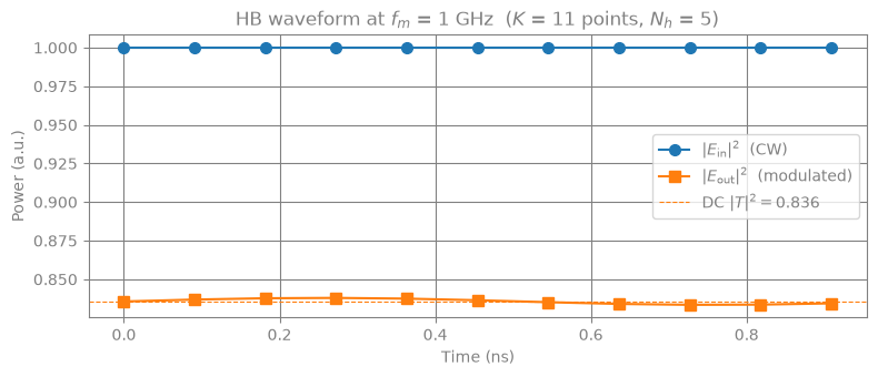
P_out oscillation amplitude: 4.4694e-03 W (peak-to-peak power modulation)
def hb_sweep_point(freq):
    """HB solve at one modulation frequency — vmappable over freq."""
    y_time, _ = circuit_hb.hb(
        freq=freq,
        harmonics=N_harm_hb,
        y0=y_dc_hb,
        params={"Vsrc.freq": freq},
    )
    E_out = circuit_hb.port(y_time, "out")
    P_out = jnp.abs(E_out) ** 2
    return jnp.max(P_out) - jnp.min(P_out)


freqs_GHz_HB = jnp.array(freqs_GHz - 0.5 * jnp.diff(freqs_GHz)[0])  # offsetting only for visualization
sweep_freqs_hb = freqs_GHz_HB * 1e9

print(f"Running vmapped HB sweep over {len(sweep_freqs_hb)} frequencies (1–50 GHz)...")
amps_hb = jax.jit(jax.vmap(hb_sweep_point))(sweep_freqs_hb)
print("Done.")

amps_hb_np = np.array(amps_hb)
amps_hb_norm = amps_hb_np / (amps_hb_np[0] + 1e-30)
amps_hb_dB = 20.0 * np.log10(amps_hb_norm + 1e-30)

fig, ax = plt.subplots(figsize=(9, 5))

ax.plot(
    freqs_GHz,
    amps_dB,
    "o-",
    ms=7.5,
    linewidth=2.0,
    zorder=3,
    label="Transient",
)
ax.plot(
    freqs_GHz_HB,
    amps_hb_dB,
    "D--",
    ms=5,
    linewidth=1.5,
    zorder=4,
    label=f"HB vmap ({len(sweep_freqs_hb)} freqs, one XLA call, $N_h$={N_harm_hb})",
)
ax.plot(freqs_GHz, H_dB, "w-", linewidth=2.0, alpha=0.7, label="Analytic: RC × optical")
ax.plot(freqs_GHz, H_opt_dB, ":", linewidth=2.0, alpha=0.5, label=r"Optical alone: $(j\omega + 2/\tau_l)/(…)$")
ax.plot(freqs_GHz, H_RC_dB, ":", linewidth=2.0, alpha=0.5, label=f"RC alone  [$f_{{RC}}$ = {f_RC / 1e9:.0f} GHz]")

ax.axhline(-3.0, color="gray", linestyle=":", linewidth=1.5, label="−3 dB")
ax.axvline(
    abs(delta_omega_dc) / (2 * np.pi * 1e9),
    color="tab:orange",
    linestyle=":",
    linewidth=0.9,
    alpha=0.7,
    label=f"|Δf| = {abs(delta_omega_dc) / (2 * np.pi * 1e9):.0f} GHz",
)

ax.set_xlabel("Modulation frequency (GHz)")
ax.set_ylabel("Normalised EO response (dB)")
ax.set_title(
    f"EO bandwidth — HB vmap vs transient vs analytic  "
    f"($V_{{bias}}$={V_bias:.0f} V, $\\Delta\\omega\\cdot\\tau$={delta_omega_dc * tau:.1f})"
)
ax.set_xlim(freqs_GHz[0], freqs_GHz[-1])
ax.set_ylim(-15.0, 12.0)
ax.legend(fontsize=8, loc="lower left")
fig.tight_layout()
plt.show()

print("\nFreq (GHz)  | Transient (dB) | HB vmap (dB) | Analytic (dB)")
print("-" * 60)
for f, a_tr, a_hb, a_an in zip(freqs_GHz[::5], amps_dB[::5], amps_hb_dB[::5], H_dB[::5]):
    print(f"  {f:5.1f}       |   {a_tr:+6.2f}        |  {a_hb:+6.2f}       | {a_an:+6.2f}")
Running vmapped HB sweep over 10 frequencies (1–50 GHz)...


Done.
Freq (GHz)  | Transient (dB) | HB vmap (dB) | Analytic (dB)
------------------------------------------------------------
    1.0       |    +0.00        |   +0.00       |  +0.00
   44.9       |    -0.56        |   -0.35       |  -0.56
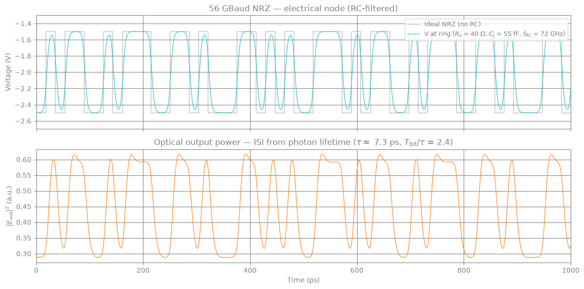
Part 4: Large-Signal NRZ Eye Diagram¤
The small-signal frequency response in Part 3 characterises the ring modulator's linear bandwidth, but it cannot predict the actual eye opening under large-signal digital modulation. Three physical effects cause eye closure and distortion that the frequency response alone cannot capture:
-
Photon lifetime ISI: The ring energy \(a(t)\) decays with time constant \(\tau \approx 7.3\,\text{ps}\), comparable to the 56 GBaud bit period \(T_{\rm bit} \approx 17.9\,\text{ps}\) (ratio \(T_{\rm bit}/\tau \approx 2.4\)). Consecutive bits see different initial ring states — a "1" after many "0"s opens differently from a "1" after many "1"s. The electrical RC bandwidth is set to \(f_{\rm RC} \approx 72\,\text{GHz} \gg f_{\rm opt} \approx 22\,\text{GHz}\) so the photon lifetime is the sole bandwidth-limiting mechanism.
-
Nonlinear Lorentzian transfer function: The ring is biased at \(\Delta\omega\cdot\tau = 1\) (on the steepest slope of the resonance), giving a large extinction ratio for a \(V_{\rm pp} = 1\,\text{V}\) swing. Even so, positive and negative half-swings produce asymmetric optical excursions because the Lorentzian is nonlinear.
-
Voltage-dependent loss (eye tilt): A small voltage-dependent round-trip amplitude \(\alpha_1 = 0.007\,\text{V}^{-1}\) makes the ring photon lifetime slightly longer at \(V_{\rm high}\) (less loss) than at \(V_{\rm low}\) (more loss). This asymmetric ISI creates a characteristic tilt in the upper and lower eye rails.
The NRZ source is modelled as a sum of sigmoid transitions — fully JAX-compatible (jittable and vmappable) — driven by a 128-bit PRBS-like pattern.
@source(ports=("p1", "p2"), states=("i_src",))
def NRZSource(
    signals: Signals,
    s: States,
    t: float,
    V_low: float = -2.5,
    V_high: float = -1.5,
    T_bit: float = 1 / 56e9,
    rise: float = 2e-12,
    bits=(0.0,) * 32,  # tuple default (hashable); pass jnp.array in practice
    t_start: float = 0.0,
) -> PhysicsReturn:
    """NRZ voltage source driven by a fixed bit pattern.

    Voltage is a sum of sigmoid step functions at each bit transition.
    ``bits`` is an array of 0/1 values.  At t < t_start the output is V_low
    (all sigmoids ≈ 0), so solve_dc called at t=0 finds the correct DC
    operating point when t_start > 0.
    """
    bits_arr = jnp.asarray(bits)
    prev = jnp.concatenate([jnp.zeros(1), bits_arr[:-1]])
    delta_bits = bits_arr - prev
    bit_times = jnp.arange(len(bits_arr)) * T_bit + t_start
    v_norm = jnp.sum(delta_bits * jax.nn.sigmoid((t - bit_times) / rise))
    v = V_low + (V_high - V_low) * v_norm
    constraint = (signals.p1 - signals.p2) - v
    return {"p1": s.i_src, "p2": -s.i_src, "i_src": constraint}, {}


# ── NRZ signal parameters ──────────────────────────────────────────────────────
T_bit_nrz = 1.0 / 56e9  # ≈ 17.86 ps per bit
N_bits_nrz = 128  # 128-bit pattern
rise_nrz = 2e-12  # 2 ps rise time (≈ 11 % of T_bit)
t_start_nrz = T_bit_nrz  # quiet preamble: ring settles at V_low before first bit

V_bias = -2.0
V_pp = 1.0
V_low_nrz = V_bias - 0.5 * V_pp
V_high_nrz = V_bias + 0.5 * V_pp

# 32-bit PRBS-like pattern tiled 4× for 128 bits
_bits32 = jnp.array(
    [1, 0, 1, 1, 0, 0, 1, 0, 1, 1, 1, 0, 0, 1, 1, 0, 1, 0, 0, 0, 1, 1, 0, 1, 0, 1, 0, 0, 1, 1, 1, 0],
    dtype=jnp.float64,
)
bits_nrz = jnp.tile(_bits32, 4)  # shape (128,)

t_end_nrz = t_start_nrz + N_bits_nrz * T_bit_nrz  # ≈ 2.3 ns total

# Voltage-dependent internal loss: alpha_v = alpha0 + alpha1_eo * V
# With reverse-bias convention (negative voltages), alpha1_eo > 0 means
# more reverse bias (more negative V) → lower alpha_v → more internal loss.
# Ring stays over-coupled (alpha_v < gamma) throughout the drive range.
alpha1_eo = 0.007  # V⁻¹  (positive; negative drive voltages give less loss at V_high)

# ── Eye-diagram circuit parameters (eye section only) ─────────────────────────
# f_RC >> f_opt so the photon lifetime is the sole bandwidth bottleneck.
R_s_eye = 40.0  # Ω   (low contact + driver resistance)
C_j_eye = 55e-15  # F   (compact depletion capacitance)
f_RC_eye = 1.0 / (2.0 * np.pi * R_s_eye * C_j_eye)
# Realistic EO coefficient for silicon PN ring at 1310 nm: ~15 GHz/V resonance shift
v_to_wr_eye = 2.0 * np.pi * 15e9  # rad/s/V

# Bias at Δω·τ = 1 (steepest slope of Lorentzian → maximum modulation depth)
# Solving 2π(f_op − f_res_eye) + v_to_wr_eye × V_bias = 1/τ for f_res_eye:
V_bias_nrz = (V_low_nrz + V_high_nrz) / 2.0  # = −2 V
detuning_eye_hz = (1.0 / tau - v_to_wr_eye * V_bias_nrz) / (2.0 * np.pi)
f_resonance_eye = float(f_operating - detuning_eye_hz)

f_opt_eye = 1.0 / (2.0 * np.pi * tau)
print(f"56 GBaud NRZ: T_bit = {T_bit_nrz * 1e12:.2f} ps,  τ = {tau * 1e12:.2f} ps  (T_bit/τ = {T_bit_nrz / tau:.1f})")
print(f"Optical bandwidth: f_opt = {f_opt_eye / 1e9:.1f} GHz  |  f_RC = {f_RC_eye / 1e9:.0f} GHz  (optically limited)")
print(f"Bias detuning: Δω·τ = 1.00 at V_bias = {V_bias_nrz:.1f} V  (f_res_eye = f_op − {detuning_eye_hz / 1e9:.1f} GHz)")
print(f"Simulation: {N_bits_nrz} bits, t_end = {t_end_nrz * 1e12:.0f} ps")
# Transmission and τ_l at each NRZ level
for _V, _label in [(V_low_nrz, "V_low"), (V_high_nrz, "V_high")]:
    _av = alpha0 + alpha1_eo * _V
    _tl = 2.0 * ng * L_ring / ((1.0 - _av**2) * 2.998e8)
    _dw = 2.0 * np.pi * detuning_eye_hz + v_to_wr_eye * _V
    _x = _dw * tau
    _A = 2.0 * tau / tau_e
    _T = np.sqrt(((1 - _A) ** 2 + _x**2) / (1 + _x**2))
    print(f"  {_label}={_V}V: α_v={_av:.4f}, τ_l={_tl * 1e12:.1f} ps, Δω·τ={_x:.2f}, |T|={_T:.3f}")

# ── Models and netlist ─────────────────────────────────────────────────────────
models_map_eye = {
    "ground": lambda: 0,
    "optical_cw": OpticalSourceStep,
    "nrz_src": NRZSource,
    "ring_eo": RingModulatorEO,
    "resistor": Resistor,
    "capacitor": Capacitor,
}

net_dict_eye = {
    "instances": {
        "GND": {"component": "ground"},
        "OptSrc": {"component": "optical_cw", "settings": {"power": 1.0}},
        "Ring": {
            "component": "ring_eo",
            "settings": {
                "ng": ng,
                "L": L_ring,
                "gamma": gamma,
                "alpha0": alpha0,
                "alpha1": alpha1_eo,  # voltage-dependent internal loss (eye diagram only)
                "f_operating": float(f_operating),
                "f_resonance": float(f_resonance_eye),
                "v_to_wr": v_to_wr_eye,
            },
        },
        "Load": {"component": "resistor", "settings": {"R": 1.0}},
        "Vsrc": {
            "component": "nrz_src",
            "settings": {
                "V_low": V_low_nrz,
                "V_high": V_high_nrz,
                "T_bit": T_bit_nrz,
                "rise": rise_nrz,
                "bits": bits_nrz,
                "t_start": t_start_nrz,
            },
        },
        "Rs": {"component": "resistor", "settings": {"R": R_s_eye}},
        "Cj": {"component": "capacitor", "settings": {"C": C_j_eye}},
    },
    "connections": {
        "GND,p1": ("OptSrc,p2", "Load,p2", "Vsrc,p2", "Cj,p2"),
        "OptSrc,p1": "Ring,p1",
        "Ring,p2": "Load,p1",
        "Vsrc,p1": "Rs,p1",
        "Rs,p2": ("Cj,p1", "Ring,v_e"),
    },
    "ports": {"in": "Ring,p1", "out": "Ring,p2", "ve": "Ring,v_e"},
}

print("\nCompiling NRZ netlist...")
circuit_eye = compile_circuit(net_dict_eye, models_map_eye, is_complex=True)

# DC at t=0: NRZSource outputs V_low (all sigmoids ≈ 0, since t_start = T_bit >> rise)
y0_nrz = circuit_eye.dc()
V_ve0 = float(jnp.real(circuit_eye.port(y0_nrz, "ve")))
T_dc_eye = float(
    jnp.abs(circuit_eye.port(y0_nrz, "out"))
    / (jnp.abs(circuit_eye.port(y0_nrz, "in")) + 1e-20)
)
print(f"DC: V_ve = {V_ve0:.3f} V  (expected {V_low_nrz:.1f} V),  |T| = {T_dc_eye:.4f}")
56 GBaud NRZ: T_bit = 17.86 ps,  τ = 7.34 ps  (T_bit/τ = 2.4)
Optical bandwidth: f_opt = 21.7 GHz  |  f_RC = 72 GHz  (optically limited)
Bias detuning: Δω·τ = 1.00 at V_bias = -2.0 V  (f_res_eye = f_op − 51.7 GHz)
Simulation: 128 bits, t_end = 2304 ps
  V_low=-2.5V: α_v=0.9515, τ_l=8.4 ps, Δω·τ=0.65, |T|=0.557
  V_high=-1.5V: α_v=0.9585, τ_l=9.8 ps, Δω·τ=1.35, |T|=0.806

Compiling NRZ netlist...


DC: V_ve = -2.500 V  (expected -2.5 V),  |T| = 0.5367
controller_nrz = diffrax.PIDController(
    rtol=1e-6,
    atol=1e-8,
    dtmax=rise_nrz / 2,  # ≤ 1 ps per step — resolves each sigmoid transition
)

print(f"Running NRZ transient simulation ({N_bits_nrz} bits at 56 GBaud, t_end = {t_end_nrz * 1e12:.0f} ps)…")
sol_nrz = circuit_eye.transient(
    t0=0.0,
    t1=t_end_nrz,
    dt0=1e-13,
    y0=y0_nrz,
    saveat=diffrax.SaveAt(ts=jnp.linspace(0.0, t_end_nrz, 32000)),
    max_steps=8_000_000,
    throw=False,
    stepsize_controller=controller_nrz,
)

if sol_nrz.result == diffrax.RESULTS.successful:
    print("Simulation successful")
else:
    print(f"Simulation ended with: {sol_nrz.result}")

ts_ps_nrz = sol_nrz.ts * 1e12
Running NRZ transient simulation (128 bits at 56 GBaud, t_end = 2304 ps)…


Simulation successful
def fold_eye(P_out, ts, t_start, T_bit, N_skip=8):
"""Fold optical power into a 3-period eye diagram, auto-centred on the crossing."""
t_eye_start = t_start + N_skip * T_bit
mask = ts >= t_eye_start
T_ps = T_bit * 1e12
P = np.array(P_out[mask])
t_raw = np.array((ts[mask] - t_eye_start) % T_bit) * 1e12
n_bins = 200
edges = np.linspace(0, T_ps, n_bins + 1)
ctrs = (edges[:-1] + edges[1:]) / 2
bidx = np.clip(np.digitize(t_raw, edges) - 1, 0, n_bins - 1)
means = np.array([P[bidx == i].mean() if np.any(bidx == i) else np.nan for i in range(n_bins)])
P_mid = (np.nanmax(means) + np.nanmin(means)) / 2
cross_ps = ctrs[np.nanargmin(np.abs(means - P_mid))]
phase = T_bit / 2 - cross_ps * 1e-12
t_fold = np.array(((ts[mask] - t_eye_start + phase) % T_bit) * 1e12)
t3 = np.concatenate([t_fold, t_fold + T_ps, t_fold + 2 * T_ps])
P3 = np.concatenate([P, P, P])
return t3, P3, T_ps
V_ve_nrz = jnp.real(circuit_eye.port(sol_nrz.ys, "ve"))
E_out_nrz = circuit_eye.port(sol_nrz.ys, "out")
P_out_nrz = jnp.abs(E_out_nrz) ** 2
t_plot_end_ps = 1000.0
t_mask = ts_ps_nrz <= t_plot_end_ps
fig, axes = plt.subplots(2, 1, figsize=(12, 6), sharex=True)
transitions_ps = (t_start_nrz + np.arange(N_bits_nrz) * T_bit_nrz) * 1e12
levels_V = V_low_nrz + (V_high_nrz - V_low_nrz) * np.array(bits_nrz)
edges_ps = np.concatenate([[0.0], transitions_ps, [t_end_nrz * 1e12]])
values_V = np.concatenate([[V_low_nrz], levels_V])
axes[0].stairs(values_V, edges_ps, color="gray", alpha=0.5, linewidth=1.0, label="Ideal NRZ (no RC)")
axes[0].plot(
ts_ps_nrz[t_mask],
np.array(V_ve_nrz[t_mask]),
color="tab:cyan",
linewidth=0.8,
label=f"V at ring ($R_s$ = {R_s_eye:.0f} Ω, $C_j$ = {C_j_eye * 1e15:.0f} fF, $f_{{RC}}$ = {f_RC_eye / 1e9:.0f} GHz)",
)
axes[0].set_ylabel("Voltage (V)")
axes[0].set_title("56 GBaud NRZ — electrical node (RC-filtered)")
axes[0].legend(loc="upper right", fontsize=9)
axes[0].set_ylim(V_low_nrz - 0.2, V_high_nrz + 0.2)
axes[0].set_xlim(0, t_plot_end_ps)
axes[1].plot(ts_ps_nrz[t_mask], np.array(P_out_nrz[t_mask]), color="tab:orange", linewidth=0.8)
axes[1].set_ylabel(r"$|E_\mathrm{out}|^2$ (a.u.)")
axes[1].set_xlabel("Time (ps)")
axes[1].set_title(
r"Optical output power — ISI from photon lifetime ($\tau \approx$ "
f"{tau * 1e12:.1f} ps, $T_{{\\rm bit}}/\\tau$ = {T_bit_nrz / tau:.1f})"
)
fig.tight_layout()
plt.show()
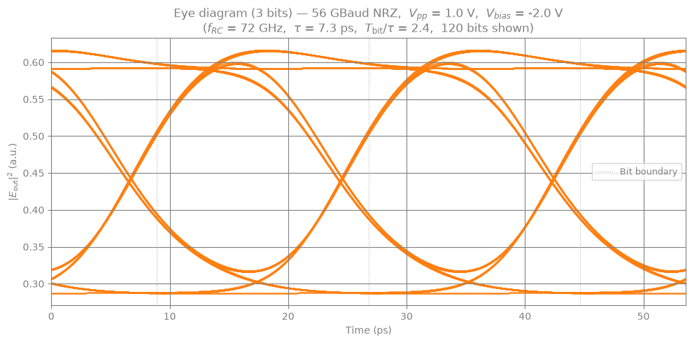
# ── Eye diagram (3 bits wide, auto-centred on optical crossing) ──────────────────────
t3_nrz, P3_nrz, T_ps_nrz = fold_eye(P_out_nrz, sol_nrz.ts, t_start_nrz, T_bit_nrz, N_skip=8)
fig, ax = plt.subplots(figsize=(10, 5))
ax.scatter(t3_nrz, P3_nrz, s=0.5, alpha=0.3, rasterized=True, color="tab:orange")
ax.set_xlabel("Time (ps)")
ax.set_ylabel(r"$|E_\mathrm{out}|^2$ (a.u.)")
ax.set_xlim(0, 3 * T_ps_nrz)
for k in range(3):
ax.axvline(
(k + 0.5) * T_ps_nrz, color="gray", linestyle=":", linewidth=0.8, alpha=0.6, label="Bit boundary" if k == 0 else None
)
ax.set_title(
f"Eye diagram (3 bits) — 56 GBaud NRZ, $V_{{pp}}$ = {V_high_nrz - V_low_nrz:.1f} V, "
f"$V_{{bias}}$ = {(V_low_nrz + V_high_nrz) / 2:.1f} V\n"
f"($f_{{RC}}$ = {f_RC_eye / 1e9:.0f} GHz, $\\tau$ = {tau * 1e12:.1f} ps, "
f"$T_{{\\rm bit}}/\\tau$ = {T_bit_nrz / tau:.1f}, {N_bits_nrz - 8} bits shown)"
)
ax.legend(fontsize=9)
fig.tight_layout()
plt.show()
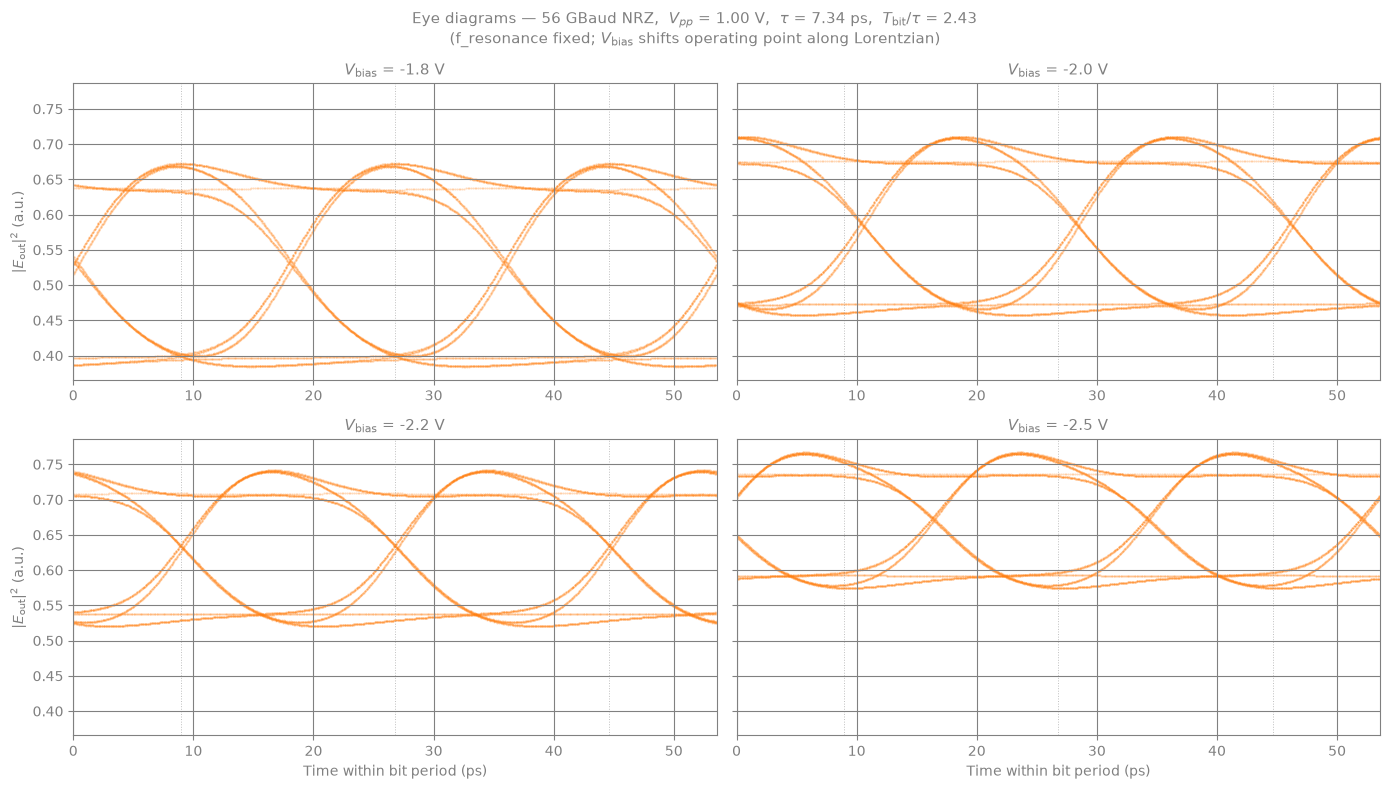
Part 5: Advanced V_bias Sweep via jax.vmap¤
With jax.vmap, we can run eye diagram simulations for multiple bias voltages in a single JIT-compiled XLA call — analogous to the HB frequency sweep in Part 3.
Each sweep point updates the NRZ voltage levels and ring resonance frequency (to keep \(\Delta\omega\cdot\tau = 1\) at the new bias), then runs the full transient simulation. The DC initial conditions are pre-computed in a Python loop.
This section is intentionally more advanced than the first-contact examples: it builds a custom compiled transient sweep, but still passes instance parameter updates through circuit.dc(...) and circuit.transient(...).
The four panels below show how the eye diagram changes as \(V_\text{bias}\) shifts the operating point along the ring Lorentzian: - Less negative bias → ring further from resonance → higher mean transmission, wider eye - More negative bias → ring closer to resonance → deeper modulation, stronger nonlinear ISI
# Pre-compute DC initial conditions for each V_bias (one Newton solve per point). This is cheap
V_bias_sweep = jnp.array([-1.75, -2.0, -2.25, -2.5])


def _eye_params(V_bias_val):
    return {
        "Vsrc.V_low": V_bias_val - 0.5 * V_pp,
        "Vsrc.V_high": V_bias_val + 0.5 * V_pp,
        "Ring.f_resonance": f_operating,
    }


y0_sweep = []
for Vb in V_bias_sweep:
    y0_sweep.append(
        circuit_eye.dc(
            params=_eye_params(float(Vb)),
            y_guess=jnp.zeros(circuit_eye.sys_size * 2, dtype=jnp.float64),
        )
    )
y0_sweep = jnp.stack(y0_sweep)  # shape (4, circuit_eye.sys_size * 2)

N_bits_vmap = 32  # 32 bits keeps per-sweep memory small
t_end_vmap = t_start_nrz + N_bits_vmap * T_bit_nrz  # ≈ 589 ps (vs 2.3 ns for Part 4)
ts_save_vmap = jnp.linspace(0.0, t_end_vmap, 4000)


def run_eye_for_vbias(V_bias_val, y0):
    """Single transient eye-diagram run, parameterised by V_bias — vmappable."""
    sol = circuit_eye.transient(
        t0=0.0,
        t1=t_end_vmap,
        dt0=1e-13,
        y0=y0,
        saveat=diffrax.SaveAt(ts=ts_save_vmap),
        max_steps=8_000_000,
        throw=False,
        params=_eye_params(V_bias_val),
        stepsize_controller=diffrax.PIDController(rtol=1e-6, atol=1e-8, dtmax=rise_nrz / 2),
    )
    return jnp.abs(circuit_eye.port(sol.ys, "out")) ** 2


print(f"Running jax.vmap over {len(V_bias_sweep)} V_bias values: {V_bias_sweep.tolist()} V")
P_out_sweep = jax.jit(jax.vmap(run_eye_for_vbias))(V_bias_sweep, y0_sweep)
print(f"Done.  Output shape: {P_out_sweep.shape}  ({P_out_sweep.shape[0]} sweeps × {P_out_sweep.shape[1]} time points)")
Running jax.vmap over 4 V_bias values: [-1.75, -2.0, -2.25, -2.5] V


Done.  Output shape: (4, 4000)  (4 sweeps × 4000 time points)
fig, axes = plt.subplots(2, 2, figsize=(14, 8), sharey=True)
axes_flat = axes.flatten()

for idx, Vb in enumerate(V_bias_sweep):
    ax = axes_flat[idx]
    t3, P3, T_ps = fold_eye(P_out_sweep[idx], ts_save_vmap, t_start_nrz, T_bit_nrz, N_skip=4)
    ax.scatter(t3, P3, s=0.3, alpha=0.25, rasterized=True, color="tab:orange")
    ax.set_xlim(0, 3 * T_ps)
    for k in range(3):
        ax.axvline((k + 0.5) * T_ps, color="gray", linestyle=":", linewidth=0.7, alpha=0.5)
    ax.set_title(f"$V_\\mathrm{{bias}}$ = {float(Vb):.1f} V", fontsize=11)
    if idx >= 2:
        ax.set_xlabel("Time within bit period (ps)")
    if idx % 2 == 0:
        ax.set_ylabel(r"$|E_\mathrm{out}|^2$ (a.u.)")

fig.suptitle(
    f"Eye diagrams — 56 GBaud NRZ,  $V_{{pp}}$ = {V_pp:.2f} V,  "
    f"$\\tau$ = {tau * 1e12:.2f} ps,  $T_\\mathrm{{bit}}/\\tau$ = {T_bit_nrz / tau:.2f}\n"
    f"(f_resonance fixed; $V_\\mathrm{{bias}}$ shifts operating point along Lorentzian)",
    fontsize=11,
)
fig.tight_layout()
plt.show()