CMOS Ring Oscillator with OSDI Models¤
Introduction¤
This example demonstrates how to simulate a CMOS ring oscillator using industry-standard compact transistor models loaded through the OSDI (Open Source Device Interface) integration.
A ring oscillator is a chain of an odd number of inverters whose output feeds back to the input. The circuit has no stable DC state — each inverter flips its successor, causing a self-sustaining oscillation whose frequency depends on the gate delay.
We use the PSP103 MOSFET model (compiled to an .osdi binary by openvaf-reloaded) and drive it through circulax's osdi_component interface, which loads the binary via the bosdi FFI layer. circulax currently requires OSDI API version 0.4.
What you will learn¤
- Loading a Verilog-A compact model via
osdi_component - Building a parameterised N-stage ring oscillator netlist
- DC initialisation with source-stepping and Gmin homotopy
- Transient simulation with fixed-step trapezoidal integration
- Extracting the oscillation frequency from the waveform
import time
from pathlib import Path

import diffrax
import equinox as eqx
import jax
import jax.numpy as jnp
import matplotlib.pyplot as plt
import numpy as np

from circulax import compile_netlist, osdi_component
from circulax.components.electronic import Resistor, SmoothPulse, VoltageSource
from circulax.solvers import analyze_circuit, setup_transient
from circulax.solvers.transient import TrapFactorizedTransientSolver

jax.config.update("jax_enable_x64", True)
1. Load the PSP103 OSDI Model¤
osdi_component takes: - osdi_path: path to the compiled .osdi binary - ports: terminal names matching the Verilog-A module declaration - default_params: base parameter values (model card); per-instance geometry is passed later through the netlist settings
The returned descriptor acts as a drop-in model class for compile_netlist. Canonical parameter names are read directly from the OSDI binary, so default_params keys are resolved case-insensitively.
We load a pre-extracted model card (psp103_defaults.json) that merges the Verilog-A source defaults with VACASK ring-oscillator overrides. The NMOS and PMOS cards are identical except for TYPE (+1 vs −1).
import json

DATA_DIR = Path("tests/data/va/psp103v4")

# Resolve relative to the repo root
for candidate in [DATA_DIR, Path.cwd().parents[1] / DATA_DIR]:
    if (candidate / "psp103.osdi").exists():
        DATA_DIR = candidate
        break

PSP103_OSDI = DATA_DIR / "psp103.osdi"

# Load the full 783-parameter model card (Verilog-A defaults + VACASK overrides).
# NMOS (TYPE=1) and PMOS (TYPE=-1) share all other parameters.
with open(DATA_DIR / "psp103_defaults.json") as f:
    nmos_defaults = json.load(f)

pmos_defaults = {**nmos_defaults, "TYPE": -1.0}

psp103n = osdi_component(
    osdi_path=str(PSP103_OSDI),
    ports=("D", "G", "S", "B"),
    default_params=nmos_defaults,
)
psp103p = osdi_component(
    osdi_path=str(PSP103_OSDI),
    ports=("D", "G", "S", "B"),
    default_params=pmos_defaults,
)

print(f"Loaded PSP103 from {PSP103_OSDI}")
print(f"  Pins:   {psp103n.ports}")
print(f"  Params: {len(psp103n.param_names)}")
Loaded PSP103 from tests/data/va/psp103v4/psp103.osdi
  Pins:   ('D', 'G', 'S', 'B')
  Params: 783
Per-instance geometry¤
Each transistor instance receives width, length, and junction-area parameters. These override the model-card defaults for that instance only.
def geom_settings(w: float, length: float, ld: float = 0.5e-6, ls: float = 0.5e-6) -> dict:
    """Per-instance MOSFET geometry."""
    return {
        "W": w, "L": length,
        "AD": w * ld, "AS": w * ls,
        "PD": 2.0 * (w + ld), "PS": 2.0 * (w + ls),
    }


NMOS_GEOM = geom_settings(10e-6, 1e-6)   # W=10 µm, L=1 µm
PMOS_GEOM = geom_settings(20e-6, 1e-6)   # W=20 µm, L=1 µm (2x for matched drive)
2. Build the Ring Oscillator Netlist¤
The circuit consists of: - VDD supply at 1.2 V - Kick source: a smooth pulse injected through a 100 kΩ resistor into node n1 to break the metastable equilibrium and start oscillation - N inverter stages: each stage has an NMOS pull-down and PMOS pull-up
The output of stage \(i\) connects to the input of stage \(i+1\), with stage \(N\) feeding back to stage 1 (the ring).
def build_ring_netlist(n_stages: int = 9):
    """Build an N-stage CMOS ring oscillator netlist."""
    if n_stages < 3 or n_stages % 2 == 0:
        raise ValueError(f"n_stages must be odd and >= 3, got {n_stages}")

    instances = {
        "Vvdd":  {"component": "vsrc",  "settings": {"V": 1.2}},
        "Vkick": {"component": "kick",  "settings": {"V": 1.0, "delay": 1e-9, "tr": 1e-9}},
        "Rkick": {"component": "r_kick", "settings": {"R": 1e5}},
    }
    connections = {
        "Vvdd,p1": "vdd,p1",     "Vvdd,p2": "GND,p1",
        "Vkick,p1": "kick_n,p1", "Vkick,p2": "GND,p1",
        "Rkick,p1": "kick_n,p1", "Rkick,p2": "n1,p1",
    }

    for stage in range(1, n_stages + 1):
        in_node  = f"n{stage}"
        out_node = f"n{stage % n_stages + 1}"
        mn, mp = f"mn{stage}", f"mp{stage}"

        instances[mn] = {"component": "nmos", "settings": NMOS_GEOM}
        instances[mp] = {"component": "pmos", "settings": PMOS_GEOM}

        connections[f"{mn},D"] = f"{out_node},p1"
        connections[f"{mn},G"] = f"{in_node},p1"
        connections[f"{mn},S"] = "GND,p1"
        connections[f"{mn},B"] = "GND,p1"
        connections[f"{mp},D"] = f"{out_node},p1"
        connections[f"{mp},G"] = f"{in_node},p1"
        connections[f"{mp},S"] = "vdd,p1"
        connections[f"{mp},B"] = "vdd,p1"

    models = {
        "nmos": psp103n, "pmos": psp103p,
        "vsrc": VoltageSource, "kick": SmoothPulse, "r_kick": Resistor,
    }

    net_dict = {
        "instances": instances,
        "connections": connections,
        "ports": {"out": "n1,p1"},
    }
    return compile_netlist(net_dict, models)
N_STAGES = 9

groups, sys_size, port_map = build_ring_netlist(N_STAGES)

print(f"Ring oscillator: {N_STAGES} stages")
print(f"System size:     {sys_size} unknowns")
print(f"Ring nodes:      {[f'n{i},p1' for i in range(1, N_STAGES + 1)]}")
Ring oscillator: 9 stages
System size:     50 unknowns
Ring nodes:      ['n1,p1', 'n2,p1', 'n3,p1', 'n4,p1', 'n5,p1', 'n6,p1', 'n7,p1', 'n8,p1', 'n9,p1']
3. DC Operating Point¤
Finding the DC operating point for a ring oscillator is tricky: the circuit is metastable (every node wants to sit at VDD/2). Circulax uses a two-phase homotopy:
Advanced OSDI convergence path
This example intentionally uses compile_netlist(), analyze_circuit(), and low-level solver methods because OSDI ring oscillators need explicit source-stepping and gmin-stepping controls. First-contact circuit examples should prefer compile_circuit() and circuit.dc()/transient().
- Source stepping — ramp VDD from 0 to 1.2 V with a high
g_leak(1e-2 S) that regularises the Jacobian - Gmin stepping — reduce
g_leakfrom 1e-2 to ~1e-12 S, letting the true device conductances take over
solver = analyze_circuit(groups, sys_size, backend="klu_split")

t0 = time.perf_counter()
high_gmin = eqx.tree_at(lambda s: s.g_leak, solver, 1e-2)
y_src = high_gmin.solve_dc_source(groups, jnp.zeros(sys_size), n_steps=20)
y0 = solver.solve_dc_gmin(groups, y_src, g_start=1e-2, n_steps=30)
dc_time = time.perf_counter() - t0

print(f"DC converged in {dc_time:.2f}s")
print(f"All finite: {bool(jnp.all(jnp.isfinite(y0)))}")
print("\nDC node voltages:")
for i in range(1, N_STAGES + 1):
    key = f"n{i},p1"
    print(f"  {key}: {float(y0[port_map[key]]):.4f} V")
DC converged in 0.97s
All finite: True

DC node voltages:
  n1,p1: 0.6606 V
  n2,p1: 0.6606 V
  n3,p1: 0.6606 V
  n4,p1: 0.6606 V
  n5,p1: 0.6606 V
  n6,p1: 0.6606 V
  n7,p1: 0.6606 V
  n8,p1: 0.6606 V
  n9,p1: 0.6592 V
4. Transient Simulation¤
We simulate 200 ns of circuit time at a fixed 50 ps timestep using the trapezoidal integrator (TrapFactorizedTransientSolver).
Trapezoidal integration is the right choice for oscillators: it is 2nd-order A-stable with zero numerical damping, so the limit-cycle frequency is preserved exactly. BDF2, by contrast, introduces L²-stable damping that pulls the oscillation frequency by ~4 %.
The kick pulse at \(t = 1\text{ ns}\) breaks the metastable state and the oscillation builds up within ~50 ns.
T_END = 200e-9     # 200 ns
DT    = 5e-11      # 50 ps
N_SAVE = 4000      # output points (50 ps resolution)

run_fn = setup_transient(groups, solver, transient_solver=TrapFactorizedTransientSolver)

saveat = diffrax.SaveAt(ts=jnp.linspace(0.0, T_END, N_SAVE))
controller = diffrax.ConstantStepSize()
max_steps = int(2 * T_END / DT)

# JIT warmup — same static shapes, tiny time window
saveat_warmup = diffrax.SaveAt(ts=jnp.linspace(0.0, 2 * DT, N_SAVE))
_ = run_fn(
    t0=0.0, t1=2 * DT, dt0=DT, y0=y0,
    saveat=saveat_warmup, max_steps=max_steps,
    stepsize_controller=controller,
).ys.block_until_ready()

# Timed run
t0 = time.perf_counter()
sol = run_fn(
    t0=0.0, t1=T_END, dt0=DT, y0=y0,
    saveat=saveat, max_steps=max_steps,
    stepsize_controller=controller,
)
sol.ys.block_until_ready()
wall = time.perf_counter() - t0

ts = np.asarray(sol.ts)
ys = np.asarray(sol.ys)
n_steps = int(T_END / DT)

print(f"Transient: {wall:.2f}s wall ({wall / n_steps * 1e6:.1f} µs/step)")
print(f"Finite:    {np.all(np.isfinite(ys))}")
Transient: 2.37s wall (593.4 µs/step)
Finite:    True
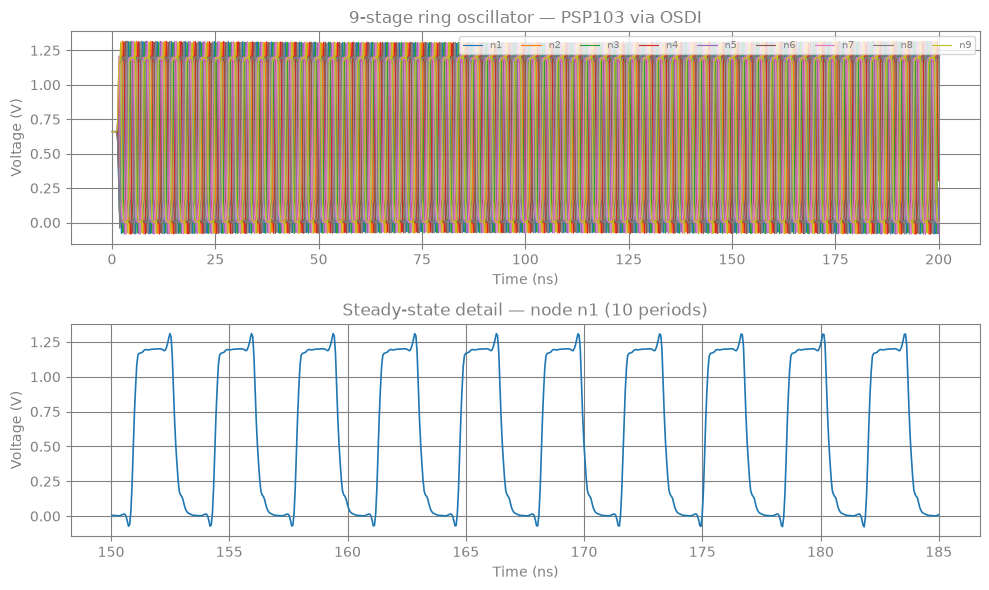
5. Output Waveforms¤
Plot the voltage at every ring node. Successive stages are phase-shifted by \(\pi / N\) — the signature pattern of a ring oscillator.
fig, axes = plt.subplots(2, 1, figsize=(10, 6))

# Full waveform — all stages
ax = axes[0]
for i in range(1, N_STAGES + 1):
    v = ys[:, port_map[f"n{i},p1"]]
    ax.plot(ts * 1e9, v, linewidth=0.8, label=f"n{i}")
ax.set_xlabel("Time (ns)")
ax.set_ylabel("Voltage (V)")
ax.set_title(f"{N_STAGES}-stage ring oscillator — PSP103 via OSDI")
ax.legend(ncol=N_STAGES, fontsize=7, loc="upper right")

# Zoom on steady-state — node n1, ~10 periods
ax = axes[1]
v1 = ys[:, port_map["n1,p1"]]
t_zoom_start = 150e-9
t_zoom_end = t_zoom_start + 35e-9  # ~10 periods at ~3.5 ns/period
mask = (ts >= t_zoom_start) & (ts <= t_zoom_end)
ax.plot(ts[mask] * 1e9, v1[mask], linewidth=1.2, color="C0")
ax.set_xlabel("Time (ns)")
ax.set_ylabel("Voltage (V)")
ax.set_title("Steady-state detail — node n1 (10 periods)")

fig.tight_layout()
plt.show()
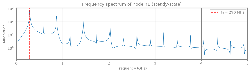
6. Oscillation Frequency¤
We extract the frequency two ways:
- Zero-crossing — interpolate rising mid-level crossings and compute the median period
- FFT — find the dominant spectral peak
Both methods ignore the first 50 ns (startup transient).
def freq_from_crossings(t: np.ndarray, x: np.ndarray) -> float:
    """Rising mid-level zero-crossing frequency."""
    centered = x - x.mean()
    rising = np.where(np.diff(np.sign(centered)) > 0)[0]
    if len(rising) < 3:
        return float("nan")
    rising = rising[1:]  # skip first partial cycle
    times = []
    for i in rising:
        x0, x1 = float(centered[i]), float(centered[i + 1])
        t0, t1 = float(t[i]), float(t[i + 1])
        times.append(t0 - x0 * (t1 - t0) / (x1 - x0))
    if len(times) < 2:
        return float("nan")
    return float(1.0 / np.median(np.diff(np.asarray(times))))


# Measure on n1, ignoring startup
v1 = ys[:, port_map["n1,p1"]]
mask = ts > 50e-9
t_ss, v_ss = ts[mask], v1[mask]

# Zero-crossing method
f_zc = freq_from_crossings(t_ss, v_ss)

# FFT method
dt_save = float(t_ss[1] - t_ss[0])
freqs = np.fft.rfftfreq(len(v_ss), d=dt_save)
power = np.abs(np.fft.rfft(v_ss - v_ss.mean()))
power[0] = 0.0
f_fft = float(freqs[np.argmax(power)])

print("Oscillation frequency:")
print(f"  Zero-crossing: {f_zc / 1e6:.1f} MHz")
print(f"  FFT peak:      {f_fft / 1e6:.1f} MHz")
print(f"  Period:         {1e9 / f_zc:.2f} ns")
print(f"  Gate delay:     {1e12 / (2 * N_STAGES * f_zc):.1f} ps")
Oscillation frequency:
  Zero-crossing: 289.6 MHz
  FFT peak:      286.6 MHz
  Period:         3.45 ns
  Gate delay:     191.8 ps
fig, ax = plt.subplots(figsize=(10, 3))

ax.semilogy(freqs / 1e9, power, linewidth=0.8)
ax.axvline(f_zc / 1e9, color="red", linestyle="--", alpha=0.7,
           label=f"f₀ = {f_zc / 1e6:.0f} MHz")
ax.set_xlabel("Frequency (GHz)")
ax.set_ylabel("Magnitude")
ax.set_title("Frequency spectrum of node n1 (steady-state)")
ax.set_xlim(0, 5)
ax.legend()
fig.tight_layout()
plt.show()
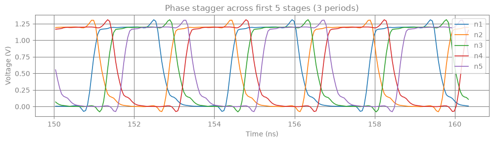
7. Phase Relationship Between Stages¤
In a ring oscillator, each stage introduces a delay of \(T / (2N)\) where \(T\) is the oscillation period. Adjacent outputs are therefore phase-shifted by \(\pi / N\) radians.
fig, ax = plt.subplots(figsize=(10, 3))

# Show 3 periods in steady state
period = 1.0 / f_zc
t_start = 150e-9
t_end = t_start + 3 * period
window = (ts >= t_start) & (ts <= t_end)

for i in range(1, min(N_STAGES + 1, 6)):  # first 5 stages for clarity
    v = ys[:, port_map[f"n{i},p1"]]
    ax.plot(ts[window] * 1e9, v[window], linewidth=1.2, label=f"n{i}")

ax.set_xlabel("Time (ns)")
ax.set_ylabel("Voltage (V)")
ax.set_title("Phase stagger across first 5 stages (3 periods)")
ax.legend(loc="upper right")
fig.tight_layout()
plt.show()
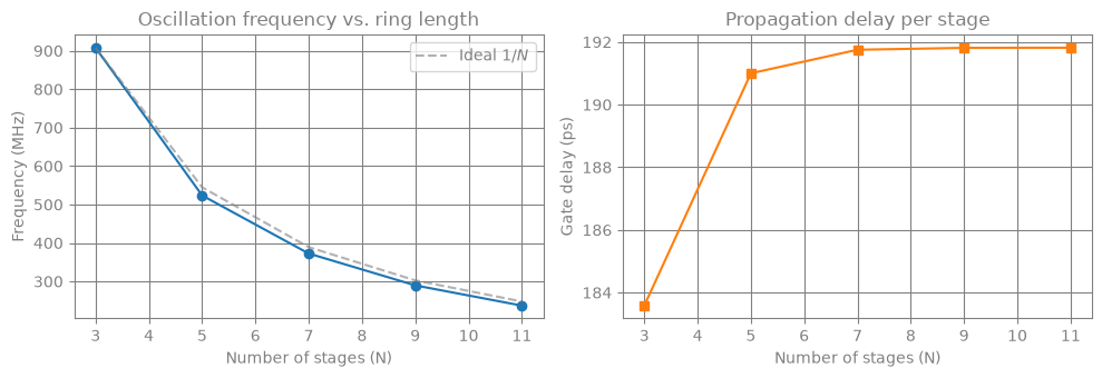
8. Frequency vs. Number of Stages¤
The oscillation frequency scales as \(f \propto 1 / (2 N \cdot t_d)\) where \(t_d\) is the propagation delay per stage. If the gate delay were constant, we would see a perfect \(1/N\) curve. In practice, loading effects and parasitic scaling cause deviations.
We sweep \(N \in \{3, 5, 7, 9, 11\}\) and measure the frequency.
stage_counts = [3, 5, 7, 9, 11]
frequencies = []
n_save_sweep = 4000

for n in stage_counts:
    grp, sz, pm = build_ring_netlist(n)
    slv = analyze_circuit(grp, sz, backend="klu_split")

    hg = eqx.tree_at(lambda s: s.g_leak, slv, 1e-2)
    ys_src = hg.solve_dc_source(grp, jnp.zeros(sz), n_steps=20)
    y_init = slv.solve_dc_gmin(grp, ys_src, g_start=1e-2, n_steps=30)

    if not bool(jnp.all(jnp.isfinite(y_init))):
        print(f"  N={n}: DC diverged")
        frequencies.append(float("nan"))
        continue

    run = setup_transient(grp, slv, transient_solver=TrapFactorizedTransientSolver)
    sa = diffrax.SaveAt(ts=jnp.linspace(0.0, T_END, n_save_sweep))
    sa_w = diffrax.SaveAt(ts=jnp.linspace(0.0, 2 * DT, n_save_sweep))
    ms = int(2 * T_END / DT)
    ctrl = diffrax.ConstantStepSize()

    _ = run(t0=0.0, t1=2*DT, dt0=DT, y0=y_init, saveat=sa_w,
            max_steps=ms, stepsize_controller=ctrl).ys.block_until_ready()

    s = run(t0=0.0, t1=T_END, dt0=DT, y0=y_init, saveat=sa,
            max_steps=ms, stepsize_controller=ctrl)
    s.ys.block_until_ready()

    t_arr = np.asarray(s.ts)
    v_arr = np.asarray(s.ys[:, pm["n1,p1"]])
    m = t_arr > 50e-9
    f = freq_from_crossings(t_arr[m], v_arr[m])
    frequencies.append(f)
    print(f"  N={n:2d}: {f / 1e6:.1f} MHz  (gate delay = {1e12 / (2 * n * f):.1f} ps)")
  N= 3: 907.9 MHz  (gate delay = 183.6 ps)


  N= 5: 523.6 MHz  (gate delay = 191.0 ps)


  N= 7: 372.5 MHz  (gate delay = 191.8 ps)


  N= 9: 289.6 MHz  (gate delay = 191.8 ps)


  N=11: 237.0 MHz  (gate delay = 191.8 ps)
stage_arr = np.array(stage_counts, dtype=float)
freq_arr = np.array(frequencies)
valid = np.isfinite(freq_arr)

fig, (ax1, ax2) = plt.subplots(1, 2, figsize=(10, 3.5))

# Frequency vs N
ax1.plot(stage_arr[valid], freq_arr[valid] / 1e6, "o-", linewidth=1.5, markersize=6)
# Ideal 1/N reference (normalised to N=3)
if valid[0]:
    f_ref = freq_arr[0]
    n_ref = stage_arr[0]
    ax1.plot(stage_arr[valid], f_ref * n_ref / stage_arr[valid] / 1e6,
             "--", color="gray", alpha=0.6, label=r"Ideal $1/N$")
    ax1.legend()
ax1.set_xlabel("Number of stages (N)")
ax1.set_ylabel("Frequency (MHz)")
ax1.set_title("Oscillation frequency vs. ring length")

# Gate delay vs N
gate_delays = 1e12 / (2 * stage_arr[valid] * freq_arr[valid])  # in ps
ax2.plot(stage_arr[valid], gate_delays, "s-", color="C1", linewidth=1.5, markersize=6)
ax2.set_xlabel("Number of stages (N)")
ax2.set_ylabel("Gate delay (ps)")
ax2.set_title("Propagation delay per stage")

fig.tight_layout()
plt.show()
Summary¤
This notebook demonstrated:
- OSDI model loading via
osdi_component— any Verilog-A model compiled by openvaf-reloaded can be used as a circulax component with zero code generation - Ring oscillator physics — the startup kick, self-sustaining oscillation, and \(\pi/N\) phase stagger between stages
- Frequency extraction from both zero-crossings and FFT
- Scaling behaviour — oscillation frequency vs. number of stages follows the expected \(1/N\) trend with a weakly N-dependent gate delay
The OSDI path through bosdi provides C-speed device evaluation while retaining the full flexibility of circulax's JAX-based solver stack — DC homotopy, implicit transient integration, and sparse KLU linear algebra.