A reduced transmission line from RLGC data¤
Build a compact, transient-capable two-port from RLGC per metre versus frequency. The factory evaluates the uniform distributed line, vector-fits its S-parameters, and checks held-out accuracy, stable poles and sampled passivity.
The returned rational circuit is causal. This is not a causality certificate for arbitrary input curves, and sampled passivity is not a global certificate. Inconsistent data or an inadequate fit raises an error.
Use this approach for an unloaded uniform line with no internal taps. Use rlgc_transmission_line instead when junctions or other devices must load intermediate sections, as in the traveling-wave MZM tutorial.
The convenience component factory is:
from circulax.components import reduced_rlgc_transmission_line
line = reduced_rlgc_transmission_line(f, R=r, L=l, G=g, C=c, length=2e-3)
Here we retain the coefficients as well so we can inspect the approximation.
# Copyright 2026 Circulax contributors

from pathlib import Path

import jax
import jax.numpy as jnp
import matplotlib.pyplot as plt
import numpy as np

from circulax import compile_circuit
from circulax.components.electronic import WAVE_PWL, Resistor, WaveformVoltageSource
from circulax.fitting import ModelFitOptions, circuit_from_coefficients, fit_rlgc, rlgc_sparameters

jax.config.update("jax_enable_x64", True)
plt.rcParams.update({"figure.figsize": (10, 3.5), "axes.grid": True})

# Retained from the earlier voltage-integration validation: bare-electrode
# scikit-rf DefinedAEpTandZ0 medium (ep_r=4.04, tanD=0.11, A=0.0009,
# f_A=1 Hz, f_ep=20 GHz, Djordjevic-Svensson dielectric model, Zc=60 ohms).
data_path = Path("data/dispersive_line_rlgc.npz")
if not data_path.is_file():
    data_path = Path("examples/electrical") / data_path
with np.load(data_path) as data:
    selected = (data["frequency_hz"] == 0) | ((data["frequency_hz"] >= 1e6) & (data["frequency_hz"] <= 60e9))
    f = data["frequency_hz"][selected]
    rlgc = {
        key: data[name][selected]
        for key, name in (
            ("R", "R_ohm_per_m"),
            ("L", "L_H_per_m"),
            ("G", "G_S_per_m"),
            ("C", "C_F_per_m"),
        )
    }
length, z0 = 2e-3, 50.0
Fit the two-port¤
RLGC inputs may be scalars, sampled arrays or functions of frequency in Hz. Their units are Ω/m, H/m, S/m and F/m. Length is in metres; z0 is the port reference impedance, not the line's characteristic impedance.
For \(s=j2\pi f\), the distributed model uses \(Z'=R+sL\), \(Y'=G+sC\), \(\gamma=\sqrt{Z'Y'}\) and the exact uniform-line ABCD matrix. It does not assume constant characteristic impedance or spatially discretize the line.
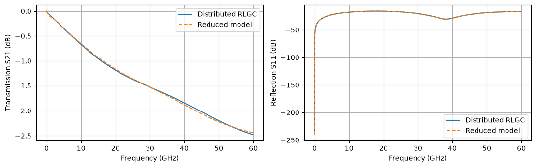
The default fit enforces sampled passivity and reserves every fifth interior sample for validation. No active integrated-voltage monitor is included. Refitting is necessary if length or RLGC changes.
For these dispersive samples, use two real poles and four complex-conjugate pairs. This ten-pole fit meets the requested accuracy after passivity enforcement. The default factory selects the order automatically; prescribed order is available when the automatic result does not meet the post-enforcement limits.
reference = rlgc_sparameters(f, **rlgc, length=length, z0=z0)
options = ModelFitOptions(vector_fit_order=(2, 4), enforce_passivity=True)
coefficients = fit_rlgc(f, **rlgc, length=length, z0=z0, options=options)
line = circuit_from_coefficients(coefficients, name="UniformLine")
print(f"Rational poles: {len(coefficients.poles)}; circuit unknowns: {line.sys_size}")
print(f"Held-out NRMSE: {coefficients.metadata['validation']['validation_nrmse']:.3%}")
print(f"Wider-grid maximum singular value: {coefficients.metadata['passivity_grid_maximum_singular_value']:.6f}")
assert np.all(coefficients.poles.real < 0)

prediction = coefficients.evaluate(f)
fig, axes = plt.subplots(1, 2, figsize=(11, 3.5))
for ax, port, label in zip(axes, (1, 0), ("Transmission S21", "Reflection S11"), strict=True):
    ax.plot(f / 1e9, 20 * np.log10(np.maximum(abs(reference[:, port, 0]), 1e-12)), label="Distributed RLGC")
    ax.plot(f / 1e9, 20 * np.log10(np.maximum(abs(prediction[:, port, 0]), 1e-12)), "--", label="Reduced model")
    ax.set(xlabel="Frequency (GHz)", ylabel=f"{label} (dB)")
    ax.legend()
plt.tight_layout()
plt.show()
# Check that the component realization preserves the fitted S response.
check_f = jnp.asarray(f[::40])
np.testing.assert_allclose(line.sp(ports=["p1", "p2"], freqs=check_f, z0=z0), coefficients.evaluate(np.asarray(check_f)), atol=1e-7)
/home/runner/work/circulax/circulax/circulax/fitting/api.py:536: UserWarning: The fitted network is passive, but the vector fit is not passive. Consider running `passivity_enforce()` to enforce passivity before using this model.
  fitter.vector_fit(n_poles_real=real, n_poles_cmplx=pairs, parameter_type="s", fit_constant=True, fit_proportional=False)


Rational poles: 10; circuit unknowns: 23
Held-out NRMSE: 0.413%
Wider-grid maximum singular value: 0.999999
Connect it to a source and load¤
The compiled line exposes p1 and p2, referenced to ground. Register it in a parent circuit just like another Circulax component. This example uses a finite-rise 1 V pulse, with 50 Ω source and load resistors.
net = {
    "instances": {
        "GND": {"component": "ground"},
        "LINE": {"component": "line"},
        "VS": {
            "component": "drive",
            "settings": {
                "kind": WAVE_PWL,
                "pwl_t": jnp.array([0, 20, 30, 80, 90, 300]) * 1e-12,
                "pwl_v": jnp.array([0, 0, 1, 1, 0, 0]),
            },
        },
        "RS": {"component": "R", "settings": {"R": z0}},
        "RL": {"component": "R", "settings": {"R": z0}},
    },
    "connections": {
        "VS,p1": "RS,p1",
        "VS,p2": "GND,p1",
        "RS,p2": "LINE,p1",
        "LINE,p2": "RL,p1",
        "RL,p2": "GND,p1",
    },
    "ports": {"input": "LINE,p1", "output": "LINE,p2"},
}
circuit = compile_circuit(net, {"line": line, "R": Resistor, "drive": WaveformVoltageSource}, is_complex=True)
times = jnp.linspace(0, 300e-12, 601)
solution = circuit.transient(t0=0.0, t1=300e-12, dt0=0.5e-12, saveat=times, max_steps=620, throw=True)
output = np.asarray(circuit.port(solution.ys, "output")).real
assert np.isfinite(output).all()
np.testing.assert_allclose(output[np.asarray(times) <= 20e-12], 0, atol=1e-10)
for port in ("input", "output"):
    plt.plot(np.asarray(times) * 1e12, np.asarray(circuit.port(solution.ys, port)).real, label=port)
plt.xlabel("Time (ps)")
plt.ylabel("Line-port voltage (V)")
plt.legend()
plt.show()
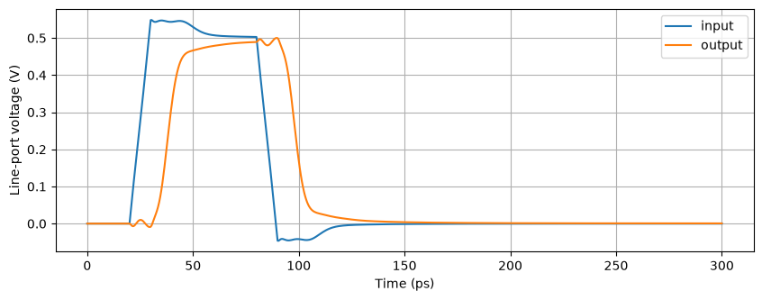
Change the frequency band, line length or RLGC data and refit. Check the error limits against your application; a compact fit is only validated over its specified band. The finite-band rational approximation does not reproduce an exact hard propagation wavefront.
ModelFitOptions can specify order and accuracy, or consistent native port delays through delay_mode="supplied" / "infer". Delay separation can reduce the rational order for suitable low-reflection lines; it is not valid to remove arbitrary phase from reflections. See the delay-fitting tutorial.
Use coefficients.save("line.npz") to retain a fit, then ModelCoefficients.load(...) and circuit_from_coefficients(...) to reuse it without fitting again.