A differentiable SOA circuit: design and electrical bandwidth¤
Build a diode-driven semiconductor optical amplifier (SOA), batch pulse simulations with JAX, and optimize its length. Then measure the small-signal electrical link MZM → fixed-current SOA → photodetector using Circuit.small_signal().
These are illustrative device parameters, not a calibrated process model. The main study uses zero passive optical loss. Heating, reflections, transport/capture dynamics, spectral gain dispersion, and ASE depletion are omitted. The optical envelope uses a moving time coordinate, with no propagation delay.
%matplotlib inline
import time
from functools import partial

import jax

jax.config.update("jax_enable_x64", True)
import jax.numpy as jnp
import matplotlib.pyplot as plt
import numpy as np

from circulax import compile_circuit
from circulax.components.base_component import PhysicsReturn, Signals, source
from circulax.components.electronic import Resistor, VoltageSource
from circulax.components.soa import SemiconductorOpticalAmplifier, soa_scales

plt.rcParams.update({"figure.figsize": (11, 4), "axes.grid": True, "grid.alpha": 0.2, "figure.constrained_layout.use": True})
length_um = 600.0
reference_current_a = 0.080  # At the 600 µm reference length.
lifetime_s = 280e-12
alpha_h = 3.5
wavelength_nm = 1540.0
bias_v = 1.8 * 0.02585 * np.log1p(reference_current_a / 1e-12) + 5 * reference_current_a
_, _, saturation_energy = map(float, soa_scales(wavelength_nm=wavelength_nm))
print("JAX", jax.__version__, "| backend:", jax.default_backend(), "| devices:", jax.devices())
print(f"Reference: {length_um:g} µm, {reference_current_a * length_um / 600 * 1e3:g} mA, tau={lifetime_s * 1e12:g} ps")
print(f"Saturation energy {saturation_energy * 1e12:.3f} pJ")
JAX 0.7.2 | backend: cpu | devices: [CpuDevice(id=0)]
Reference: 600 µm, 80 mA, tau=280 ps
Saturation energy 1.433 pJ
1. One diode and one gain reservoir¤
The electrical path is anode → series resistance → diode || junction capacitance → cathode. Diode conduction current pumps the gain reservoir; displacement current does not. Contact area scales with length, so diode saturation current and capacitance scale with length and vertical series resistance scales inversely.
For active volume \(V_a=wdL\) and modal differential gain \(a_m=\Gamma a\),
The output field is \(A_{out}=A_{in}\exp[(1-j\alpha_H)h/2]\). Circulax expresses this ODE as a storage term in \(F+dQ/dt=0\). Optical depletion does not feed back into the electrical voltage.
Our design vector is [length (µm), pump-density multiplier, input pulse energy (pJ)]. A multiplier of one means 80 mA at 600 µm, with total current proportional to length. Thus changing length holds current density fixed. Lifetime and Henry factor stay fixed throughout the pulse design study.
@source(ports=("p1", "p2"), states=("i_src",), holomorphic=True)
def pulse_source(
    signals: Signals,
    t: float,
    pulse_energy: float = 0.0,
    pulse_center: float = 60e-12,
    pulse_fwhm: float = 8e-12,
) -> PhysicsReturn:
    sigma = pulse_fwhm / jnp.sqrt(8 * jnp.log(2.0))
    pulse = pulse_energy / (sigma * jnp.sqrt(2 * jnp.pi)) * jnp.exp(-0.5 * ((t - pulse_center) / sigma) ** 2)
    # A negligible power floor keeps sqrt derivatives finite in dark tails.
    field = jnp.sqrt(pulse + 1e-30)
    return {"p1": signals.i_src, "p2": -signals.i_src, "i_src": signals.p1 - signals.p2 - field}, {}


netlist = {
    "instances": {
        "SOA": {"component": "soa"},
        "BIAS": {"component": "bias"},
        "LIGHT": {"component": "light"},
        "LOAD": {"component": "load", "settings": {"R": 1.0}},
        "GND": {"component": "ground"},
    },
    "connections": {
        "GND,p1": ("BIAS,p2", "LIGHT,p2", "LOAD,p2", "SOA,cathode"),
        "BIAS,p1": "SOA,anode",
        "LIGHT,p1": "SOA,optical_in",
        "SOA,optical_out": "LOAD,p1",
    },
    "ports": {"input": "SOA,optical_in", "output": "SOA,optical_out"},
}
circuit = compile_circuit(
    netlist,
    {"soa": SemiconductorOpticalAmplifier, "bias": VoltageSource, "light": pulse_source, "load": Resistor, "ground": lambda: 0},
    is_complex=True,
    backend="dense",
    rtol=1e-9,
    atol=1e-11,
)
base = {
    "SOA.lifetime_s": lifetime_s,
    "SOA.alpha_h": alpha_h,
    "SOA.saturation": 1.0,
    "SOA.wavelength_nm": wavelength_nm,
}
# The circuit topology is built once. Only numeric parameters change.
def design_params(design):
    length, density, energy_pj = design
    contact_scale = length / 600.0
    current = reference_current_a * contact_scale * density
    voltage = 1.8 * 0.02585 * jnp.log1p(current / (1e-12 * contact_scale)) + 5 / contact_scale * current
    return {
        **base,
        "SOA.length_um": length,
        "BIAS.V": voltage,
        "LIGHT.pulse_energy": energy_pj * 1e-12,
    }


@partial(jax.jit, static_argnames=("duration", "step"))
def solve_design(design, *, duration=240e-12, step=0.25e-12):
    params = design_params(design)
    times = jnp.linspace(0.0, duration, round(duration / step) + 1)
    initial = circuit.dc(params={**params, "LIGHT.pulse_energy": 0.0})
    sol = circuit.transient(
        t0=0.0, t1=duration, dt0=step, y0=initial, saveat=times, params=params, max_steps=round(duration / step) + 16
    )
    return {
        "time": sol.ts,
        "input": circuit.port(sol.ys, "input"),
        "output": circuit.port(sol.ys, "output"),
    }


def pulse_metrics(result):
    # Integrate optical power; the source contains only the isolated pulse.
    pin, pout = jnp.abs(result["input"]) ** 2, jnp.abs(result["output"]) ** 2
    t = result["time"]
    ein, eout = jnp.trapezoid(pin, t), jnp.trapezoid(pout, t)
    return jnp.array([10 * jnp.log10(eout / ein), eout * 1e12])


def evaluate(design):
    return pulse_metrics(solve_design(design))


reference_design = jnp.array([length_um, 1.0, 0.25])
batched_metrics = jax.jit(jax.vmap(evaluate))
2. Batch designs, then measure warm execution¤
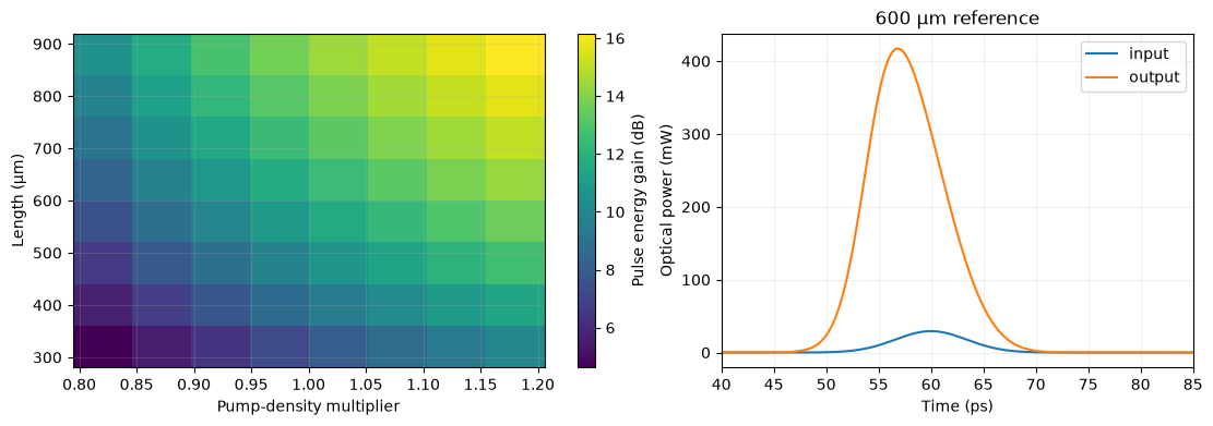
vmap adds independent design cases to the same compiled circuit; jit compiles their numerical work. The grid fixes the input pulse energy at 0.25 pJ and varies length and pump density. Inspect one waveform alongside the energy map: carrier depletion reshapes the pulse, so energy gain alone is not a complete pulse-quality metric.
The timing comparison uses identical designs, tolerances, and outputs. Both paths synchronize the device before stopping the clock. First-call time includes compilation; warm time reuses compiled executables. Batching can reduce dispatch overhead and vectorize numerical work, but its benefit depends on hardware and workload. A different batch shape can trigger compilation.
lengths = jnp.linspace(320.0, 880.0, 8)
densities = jnp.linspace(0.82, 1.18, 8)
ll, dd = jnp.meshgrid(lengths, densities, indexing="ij")
designs = jnp.stack([ll.ravel(), dd.ravel(), jnp.full(ll.size, 0.25)], axis=1)
start = time.perf_counter()
metrics = batched_metrics(designs)
metrics.block_until_ready()
print(f"{len(designs)} nonlinear transients, first call including compilation: {time.perf_counter() - start:.3f} s")
assert np.isfinite(metrics).all()
reference = solve_design(reference_design)
fig, axes = plt.subplots(1, 2, figsize=(11, 3.8))
image = axes[0].pcolormesh(densities, lengths, np.asarray(metrics[:, 0]).reshape(ll.shape), shading="nearest")
fig.colorbar(image, ax=axes[0], label="Pulse energy gain (dB)")
axes[0].set(xlabel="Pump-density multiplier", ylabel="Length (µm)")
for port in ["input", "output"]:
    axes[1].plot(reference["time"] * 1e12, jnp.abs(reference[port]) ** 2 * 1e3, label=port)
axes[1].set(xlim=(40, 85), xlabel="Time (ps)", ylabel="Optical power (mW)", title="600 µm reference")
axes[1].legend()
plt.show()

# Check independent cases and one finer timestep before trusting the grid.
for idx in [0, len(designs) - 1]:
    np.testing.assert_allclose(metrics[idx], evaluate(designs[idx]), rtol=2e-7, atol=1e-8)
refined = pulse_metrics(solve_design(designs[-1], step=0.125e-12))
np.testing.assert_allclose(metrics[-1, 1], refined[1], rtol=0.003)
64 nonlinear transients, first call including compilation: 6.085 s
benchmark_designs = designs[jnp.linspace(0, len(designs) - 1, 24).astype(int)]
scalar_metrics = jax.jit(evaluate)
# A separate wrapper makes its first compilation visible in this benchmark.
benchmark_batch = jax.jit(jax.vmap(evaluate))

start = time.perf_counter()
scalar_metrics(benchmark_designs[0]).block_until_ready()
scalar_first = time.perf_counter() - start
start = time.perf_counter()
benchmark_batch(benchmark_designs).block_until_ready()
batch_first = time.perf_counter() - start


def measure(call, repeats=3):
    timings = []
    for _ in range(repeats):
        start = time.perf_counter()
        jax.block_until_ready(call())
        timings.append(time.perf_counter() - start)
    return float(np.median(timings))


serial_result = jnp.stack([scalar_metrics(d) for d in benchmark_designs])
batch_result = benchmark_batch(benchmark_designs)
np.testing.assert_allclose(serial_result, batch_result, rtol=2e-7, atol=1e-8)
serial_seconds = measure(lambda: jnp.stack([scalar_metrics(d) for d in benchmark_designs]))
batch_seconds = measure(lambda: benchmark_batch(benchmark_designs))
grid_seconds = measure(lambda: batched_metrics(designs))
print(f"Scalar first call: {scalar_first:.3f} s; {len(benchmark_designs)}-case batch first call: {batch_first:.3f} s")
print(f"Warm serial loop: {serial_seconds:.4f} s; warm batch: {batch_seconds:.4f} s")
print(f"Measured serial/batch ratio: {serial_seconds / batch_seconds:.2f}x")
print(f"Full warm grid: {len(designs)} cases in {grid_seconds:.4f} s ({len(designs) / grid_seconds:.1f} cases/s)")
Scalar first call: 2.112 s; 24-case batch first call: 4.774 s
Warm serial loop: 0.6984 s; warm batch: 0.2058 s
Measured serial/batch ratio: 3.39x
Full warm grid: 64 cases in 0.4624 s (138.4 cases/s)
3. Gradient descent chooses the length¤
Choose a target output pulse energy of 3 pJ and minimize
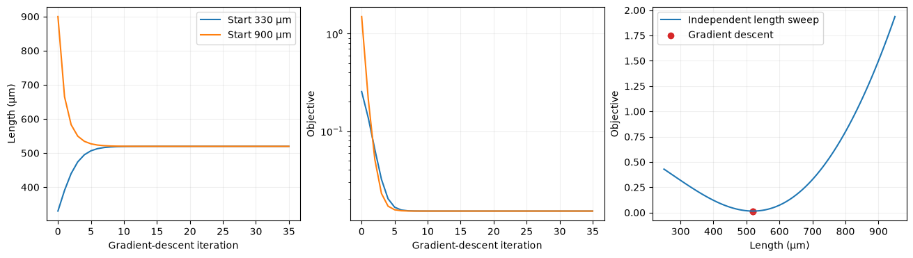
The footprint penalty favors slightly shorter devices over exact energy matching. This soft objective is not a hard minimum-length constraint. Current density and input pulse energy stay fixed; allowed lengths are 250–950 µm.
A central finite difference first checks the local derivative through the transient. Then value_and_grad, lax.scan, and vmap run 36 projected gradient steps from two starting lengths. An independent length sweep checks the final objective.
target_energy_pj = 3.0


def length_loss(normalized_length):
    design = reference_design.at[0].set(600 * normalized_length)
    output_energy = evaluate(design)[1]
    return (output_energy / target_energy_pj - 1) ** 2 + 0.02 * normalized_length**2


length_value_grad = jax.value_and_grad(length_loss)

# Derivative is with respect to L / 600 µm, keeping its scale near one.
epsilon = 2e-3
_, gradient = length_value_grad(1.0)
finite_difference = (length_loss(1 + epsilon) - length_loss(1 - epsilon)) / (2 * epsilon)
np.testing.assert_allclose(gradient, finite_difference, rtol=0.015, atol=0.003)
print(f"Length gradient: AD {gradient:.6f}, finite difference {finite_difference:.6f}")


def descend(initial_length):
    def step(x, _):
        loss, gradient = length_value_grad(x)
        return jnp.clip(x - 0.08 * gradient, 250 / 600, 950 / 600), jnp.array([x * 600, loss, gradient])

    final, history = jax.lax.scan(step, initial_length / 600, xs=None, length=36)
    return final * 600, history


optimize_lengths = jax.jit(jax.vmap(descend))
start = time.perf_counter()
optimized, history = optimize_lengths(jnp.array([330.0, 900.0]))
jax.block_until_ready(optimized)
print(f"Compiled optimization including first execution: {time.perf_counter() - start:.3f} s")
start = time.perf_counter()
jax.block_until_ready(optimize_lengths(jnp.array([330.0, 900.0])))
print(f"Warm 36-step optimization, two starts: {time.perf_counter() - start:.3f} s")
check_lengths = jnp.linspace(250, 950, 81)
check_losses = jax.jit(jax.vmap(length_loss))(check_lengths / 600)
final_losses = jax.vmap(length_loss)(optimized / 600)
np.testing.assert_allclose(optimized[0], optimized[1], atol=1.0)
assert np.all(np.asarray(final_losses) < np.min(check_losses) + 0.001)
assert np.all(np.asarray(final_losses) < np.asarray(history[:, 0, 1]))
fig, axes = plt.subplots(1, 3, figsize=(13, 3.6))
for k, initial in enumerate([330, 900]):
    axes[0].plot(np.asarray(history[k, :, 0]), label=f"Start {initial} µm")
    axes[1].semilogy(np.asarray(history[k, :, 1]))
axes[0].set(xlabel="Gradient-descent iteration", ylabel="Length (µm)")
axes[0].legend()
axes[1].set(xlabel="Gradient-descent iteration", ylabel="Objective")
axes[2].plot(check_lengths, check_losses, label="Independent length sweep")
axes[2].scatter(optimized, final_losses, color="tab:red", label="Gradient descent")
axes[2].set(xlabel="Length (µm)", ylabel="Objective")
axes[2].legend()
plt.show()
for optimum in np.asarray(optimized):
    d = reference_design.at[0].set(optimum)
    print(f"Length {optimum:.2f} µm → output {float(evaluate(d)[1]):.3f} pJ; target {target_energy_pj:g} pJ")
Length gradient: AD 0.896826, finite difference 0.896830


Compiled optimization including first execution: 33.088 s


Warm 36-step optimization, two starts: 16.444 s
Length 519.73 µm → output 2.970 pJ; target 3 pJ
Length 519.73 µm → output 2.970 pJ; target 3 pJ
4. Measure electrical S21 with a fixed SOA pump¤
The RF source drives a matched 50 Ω MZM input. A buffered Bessel3 electrical-drive filter (35 GHz default) precedes the static quadrature MZI transfer (\(V_\pi=4\) V). It represents compact modulator dynamics; it is not a passive RF network. An independent DC current source pumps the SOA, and an ideal square-law detector drives a 50 Ω receiver.
With equal 50 Ω reference impedances,
The factor of two accounts for source voltage division. small_signal() linearizes the CW circuit, including optical real/imaginary coordinates and the carrier reservoir. The SOA current is not RF-modulated.
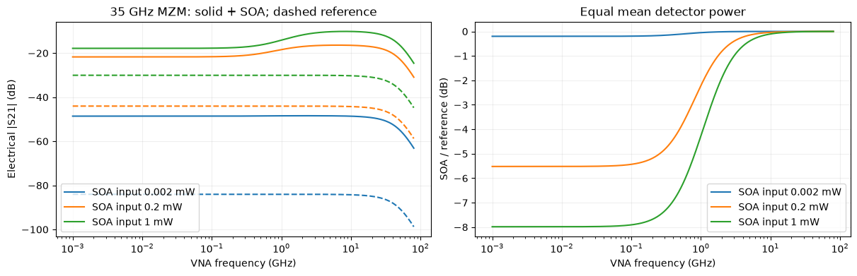
Absolute S21 includes average optical amplification. To isolate modulation-depth changes, attenuate the SOA output until its mean detector power matches the MZM-only reference, then divide the two complex responses. Both paths have the same modulator filter, which cancels in this equal-power de-embedding. Normalizing each path to its own low-frequency response would hide carrier suppression.
Slow intensity modulation depletes carriers in opposition to the input modulation. At high frequency the carriers cannot follow, so this suppression weakens; the modulator filter still rolls off. For zero passive loss an independent reservoir benchmark is
The plots distinguish this low-frequency shelf from high-frequency MZM rolloff. A smooth shelf is the prediction of this model, not a calibrated explanation for a sharp experimental notch. Optical filtering, dispersion, modulator chirp, receiver bandwidth, and calibration can change a measured link.
from circulax.components.base_component import component
from circulax.components.electronic import CurrentSource
from circulax.components.filters import Bessel3
from circulax.components.photonic import OpticalSource

mzi_filter_f3db = 35e9


@component(ports=("ein", "eout", "control"), states=("i_out",), holomorphic=False)
def vna_modulator(signals: Signals, vpi: float = 4.0, bias_phase: float = np.pi / 2) -> PhysicsReturn:
    phase = bias_phase + jnp.pi * jnp.real(signals.control) / vpi
    field = signals.ein * jnp.cos(phase / 2)
    return {"ein": signals.ein, "control": 0.0, "eout": signals.i_out, "i_out": signals.eout - field}, {}


@component(ports=("ein", "eout"), states=("i_out",), holomorphic=True)
def vna_attenuator(signals: Signals, transmission: float = 1.0) -> PhysicsReturn:
    return {"ein": signals.ein, "eout": signals.i_out, "i_out": signals.eout - jnp.sqrt(transmission) * signals.ein}, {}


@component(ports=("ein", "out", "ground"), holomorphic=False)
def vna_detector(signals: Signals, responsivity: float = 0.8) -> PhysicsReturn:
    current = responsivity * jnp.abs(signals.ein) ** 2
    return {"ein": signals.ein, "out": -current, "ground": current}, {}


def vna_fixture(include_soa):
    instances = {
        "GND": {"component": "ground"},
        "LASER": {"component": "laser"},
        "RF": {"component": "voltage"},
        "R_SOURCE": {"component": "resistor", "settings": {"R": 50.0}},
        "R_MOD": {"component": "resistor", "settings": {"R": 50.0}},
        "MZM": {"component": "mzm"},
        "MZM_BW": {"component": "bessel3", "settings": {"f3db": mzi_filter_f3db}},
        "ATT": {"component": "attenuator"},
        "PD": {"component": "detector"},
        "R_RX": {"component": "resistor", "settings": {"R": 50.0}},
    }
    ground_nodes = ["LASER,p2", "RF,p2", "R_MOD,p2", "PD,ground", "R_RX,p2"]
    connections = {
        "LASER,p1": "MZM,ein",
        "RF,p1": "R_SOURCE,p1",
        "R_SOURCE,p2": ("MZM_BW,inp", "R_MOD,p1"),
        "MZM_BW,out": "MZM,control",
        "ATT,eout": "PD,ein",
        "PD,out": "R_RX,p1",
    }
    if include_soa:
        instances.update({"SOA": {"component": "soa"}, "PUMP": {"component": "current"}})
        ground_nodes.extend(["SOA,cathode", "PUMP,p1"])
        connections.update({"PUMP,p2": "SOA,anode", "MZM,eout": "SOA,optical_in", "SOA,optical_out": "ATT,ein"})
    else:
        connections["MZM,eout"] = "ATT,ein"
    connections["GND,p1"] = tuple(ground_nodes)
    return compile_circuit(
        {"instances": instances, "connections": connections, "ports": {"receiver": "PD,out"}},
        {
            "laser": OpticalSource,
            "voltage": VoltageSource,
            "resistor": Resistor,
            "mzm": vna_modulator,
            "bessel3": Bessel3,
            "attenuator": vna_attenuator,
            "detector": vna_detector,
            "soa": SemiconductorOpticalAmplifier,
            "current": CurrentSource,
            "ground": lambda: 0,
        },
        is_complex=True,
        backend="dense",
        rtol=1e-10,
        atol=1e-12,
    )
vna_soa = vna_fixture(True)
vna_reference = vna_fixture(False)
vna_freqs = jnp.sort(jnp.r_[0.0, jnp.geomspace(1e6, 80e9, 321), mzi_filter_f3db])
vna_open_voltage = 1e-3
vna_input_powers = jnp.array([2e-6, 2e-4, 1e-3])


def vna_case(power, filter_f3db=mzi_filter_f3db):
    params = {
        "LASER.power": 2 * power,
        "MZM_BW.f3db": filter_f3db,
        "PUMP.I": reference_current_a * length_um / 600,
        "SOA.length_um": length_um,
        "SOA.lifetime_s": lifetime_s,
        "SOA.alpha_h": alpha_h,
        "SOA.wavelength_nm": wavelength_nm,
    }
    model = vna_soa.small_signal(params=params)
    result = model(freqs=vna_freqs, sources={"RF": vna_open_voltage})
    reference_model = vna_reference.small_signal(params={"LASER.power": 2 * power, "MZM_BW.f3db": filter_f3db})
    reference_result = reference_model(freqs=vna_freqs, sources={"RF": vna_open_voltage})
    gain = jnp.abs(vna_soa.port(model.y_dc, "SOA,optical_out")) ** 2 / power
    equal_power_model = vna_soa.small_signal(params={**params, "ATT.transmission": 1 / gain})
    equal_power = equal_power_model(freqs=vna_freqs, sources={"RF": vna_open_voltage})
    s21 = 2 * result.voltage("receiver") / vna_open_voltage
    s21_ref = 2 * reference_result.voltage("receiver") / vna_open_voltage
    s21_equal = 2 * equal_power.voltage("receiver") / vna_open_voltage
    junction = result.voltage("SOA,v_j")
    # DC current and its RF perturbation remain independent of optical drive.
    diode_current = 1e-12 * (length_um / 600) * jnp.expm1(jnp.real(vna_soa.port(model.y_dc, "SOA,v_j")) / (1.8 * 0.02585))
    detector_dc = vna_soa.port(equal_power_model.y_dc, "receiver")
    reference_dc = vna_reference.port(reference_model.y_dc, "receiver")
    return s21, s21_ref, s21_equal, junction, diode_current, detector_dc, reference_dc, gain


vna_results = jax.jit(jax.vmap(vna_case))(vna_input_powers)
s21, s21_reference, s21_equal, junction_rf, pump_current, detector_dc, reference_dc, vna_gains = vna_results
np.testing.assert_allclose(pump_current, reference_current_a * length_um / 600, rtol=1e-6)


def bessel_benchmark(freqs, cutoff):
    p = 1j * freqs / (cutoff / 1.7556723686812106)
    return 15 / (p**3 + 6 * p**2 + 15 * p + 15)


filter_benchmark = bessel_benchmark(vna_freqs, mzi_filter_f3db)
expected_reference_s21 = -50 * 0.8 * jnp.pi / 4 * vna_input_powers[:, None] * filter_benchmark
np.testing.assert_allclose(abs(bessel_benchmark(mzi_filter_f3db, mzi_filter_f3db)), 1 / np.sqrt(2), rtol=1e-12)
np.testing.assert_allclose(s21_reference, jnp.broadcast_to(expected_reference_s21, s21_reference.shape), rtol=1e-7, atol=1e-12)
np.testing.assert_allclose(junction_rf, 0, atol=1e-12)
np.testing.assert_allclose(detector_dc, reference_dc, rtol=1e-6, atol=1e-12)
# Compare the complete electrical measurement with the independent carrier formula.
r = 1 / lifetime_s + vna_input_powers[:, None] * vna_gains[:, None] / saturation_energy
analytic_link_ratio = 1 - vna_input_powers[:, None] * (vna_gains[:, None] - 1) / saturation_energy / (r + 2j * jnp.pi * vna_freqs)
np.testing.assert_allclose(s21_equal / s21_reference, analytic_link_ratio, rtol=2e-6, atol=1e-8)
fig, axes = plt.subplots(1, 2, figsize=(12, 3.8))
fghz = np.asarray(vna_freqs[1:]) / 1e9
for k, power in enumerate(vna_input_powers):
    label = f"SOA input {float(power) * 1e3:g} mW"
    axes[0].semilogx(fghz, 20 * np.log10(np.abs(s21[k, 1:])), color=f"C{k}", label=label)
    axes[0].semilogx(fghz, 20 * np.log10(np.abs(s21_reference[k, 1:])), "--", color=f"C{k}")
    ratio = np.asarray(s21_equal[k] / s21_reference[k])
    axes[1].semilogx(fghz, 20 * np.log10(np.abs(ratio[1:])), label=label)
    print(f"Input {float(power) * 1e3:g} mW: equal-power DC RF suppression {20 * np.log10(abs(ratio[0])):.2f} dB")
axes[0].set(
    xlabel="VNA frequency (GHz)",
    ylabel="Electrical |S21| (dB)",
    title=f"{mzi_filter_f3db / 1e9:g} GHz MZM: solid + SOA; dashed reference",
)
axes[1].set(xlabel="VNA frequency (GHz)", ylabel="SOA / reference (dB)", title="Equal mean detector power")
for ax in axes:
    ax.legend()
plt.show()
Input 0.002 mW: equal-power DC RF suppression -0.20 dB
Input 0.2 mW: equal-power DC RF suppression -5.52 dB
Input 1 mW: equal-power DC RF suppression -7.98 dB
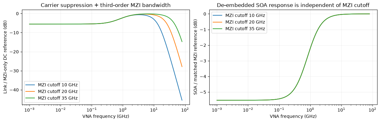
Changing only the MZM cutoff moves the high-frequency rolloff. The de-embedded SOA shelf stays fixed because optical loading and pump current are unchanged. The analytic Bessel response above also checks the complete complex reference S21, including its phase and exact −3.0103 dB cutoff.
# Vary the MZI bandwidth while holding optical loading and pump current fixed.
cutoffs = jnp.array([10e9, 20e9, 35e9])
cutoff_results = jax.jit(jax.vmap(lambda cutoff: vna_case(vna_input_powers[1], cutoff)))(cutoffs)
cutoff_reference = cutoff_results[1]
cutoff_equal = cutoff_results[2]
deembedded = cutoff_equal / cutoff_reference
np.testing.assert_allclose(deembedded, jnp.broadcast_to(deembedded[0], deembedded.shape), rtol=2e-6, atol=1e-8)
fig, axes = plt.subplots(1, 2, figsize=(12, 3.8))
for k, cutoff in enumerate(cutoffs):
    label = f"MZI cutoff {float(cutoff) / 1e9:g} GHz"
    # Normalize all curves to the matching MZI-only DC response, preserving
    # SOA suppression rather than normalizing it away at low frequency.
    combined = cutoff_equal[k] / cutoff_reference[k, 0]
    axes[0].semilogx(fghz, 20 * np.log10(np.abs(combined[1:])), label=label)
    axes[1].semilogx(fghz, 20 * np.log10(np.abs(deembedded[k, 1:])), label=label)
axes[0].set(
    xlabel="VNA frequency (GHz)",
    ylabel="Link / MZI-only DC reference (dB)",
    title="Carrier suppression + third-order MZI bandwidth",
)
axes[1].set(
    xlabel="VNA frequency (GHz)",
    ylabel="SOA / matched MZI reference (dB)",
    title="De-embedded SOA response is independent of MZI cutoff",
)
axes[0].legend()
axes[1].legend()
plt.show()
print("Bessel reference magnitude/phase, exact cutoff, and MZI-bandwidth de-embedding checks passed.")
Bessel reference magnitude/phase, exact cutoff, and MZI-bandwidth de-embedding checks passed.
Optional: when does length need spatial sections?¤
A long device does not automatically need more states. With one forward wave, linear material gain, uniform lifetime, zero passive loss, and moving time, the integrated reservoir closes exactly: stimulated extraction telescopes as \(\sum(P_{j+1}-P_j)=P_{out}-P_{in}\). Local carriers may still vary along the device.
Distributed passive loss breaks that identity: carrier extraction differs from net output-minus-input power. The component accounts for this within each constant-gain section. Compare 1, 2, 4, and 8 sections at equal total length and current density: the lossless energy is invariant, while the lossy energy should converge. Nonuniform pumping/lifetime, counterpropagating fields, and ASE depletion can also require spatial resolution.
These sections have no propagation delay. They resolve longitudinal carriers in the moving frame. Laboratory-time arrival or rapidly varying pumping needs delay/traveling-wave treatment. Each section count is a separate static circuit topology.
def segmented_fixture(sections):
    instances = {
        "BIAS": {"component": "bias"},
        "LIGHT": {"component": "light"},
        "LOAD": {"component": "load", "settings": {"R": 1.0}},
        "GND": {"component": "ground"},
    }
    for k in range(sections):
        instances[f"S{k}"] = {"component": "soa"}
    connections = {
        "GND,p1": tuple(["BIAS,p2", "LIGHT,p2", "LOAD,p2"] + [f"S{k},cathode" for k in range(sections)]),
        "BIAS,p1": tuple(f"S{k},anode" for k in range(sections)),
        "LIGHT,p1": "S0,optical_in",
        f"S{sections - 1},optical_out": "LOAD,p1",
    }
    connections.update({f"S{k},optical_out": f"S{k + 1},optical_in" for k in range(sections - 1)})
    return compile_circuit(
        {"instances": instances, "connections": connections, "ports": {"output": f"S{sections - 1},optical_out"}},
        {"soa": SemiconductorOpticalAmplifier, "bias": VoltageSource, "light": pulse_source, "load": Resistor, "ground": lambda: 0},
        is_complex=True,
        backend="dense",
        rtol=1e-9,
        atol=1e-11,
    )


long_length = 1400.0
section_counts = [1, 2, 4, 8]
section_energy = {0.0: [], 18.0: []}
for count in section_counts:
    segmented = segmented_fixture(count)

    @jax.jit
    def section_run(loss, segmented=segmented, count=count):
        params = {
            "length_um": long_length / count,
            "loss_db_per_cm": loss,
            "BIAS.V": bias_v,
            "lifetime_s": lifetime_s,
            "alpha_h": alpha_h,
            "wavelength_nm": wavelength_nm,
            "LIGHT.pulse_energy": 0.3e-12,
        }
        initial = segmented.dc(params={**params, "LIGHT.pulse_energy": 0.0})
        ts = jnp.linspace(0.0, 200e-12, 401)
        sol = segmented.transient(t0=0.0, t1=200e-12, dt0=0.5e-12, y0=initial, saveat=ts, params=params, max_steps=416)
        field = segmented.port(sol.ys, "output")
        return jnp.trapezoid(jnp.abs(field) ** 2, ts) * 1e12

    # Batch loss settings within each fixed topology.
    energy = jax.vmap(section_run)(jnp.array([0.0, 18.0]))
    for k, loss in enumerate([0.0, 18.0]):
        section_energy[loss].append(float(energy[k]))
np.testing.assert_allclose(section_energy[0.0], section_energy[0.0][0], rtol=0.003)
lossy_error_db = 10 * np.log10(np.asarray(section_energy[18.0]) / section_energy[18.0][-1])
assert abs(lossy_error_db[-2]) < 0.1
fig, ax = plt.subplots(figsize=(7, 3.5))
for loss, values in section_energy.items():
    ax.plot(section_counts, values, "o-", label=f"Passive loss {loss:g} dB/cm")
ax.set(xlabel="Number of sections", ylabel="Output pulse energy (pJ)")
ax.legend()
plt.show()
print("Lossy energy differences relative to 8 sections (dB):", lossy_error_db)
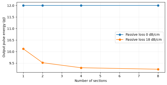
Lossy energy differences relative to 8 sections (dB): [0.39655033 0.13060814 0.0298819 0. ]
The core workflow is now reusable: compile topology once, batch numerical parameters, check local derivatives, optimize a defined metric, and linearize the resulting link at its CW operating point. Warm timings are local synchronized measurements. The independent benchmarks check numerical consistency within this illustrative model; they do not establish physical fidelity or unlimited SOA bandwidth.