TFLN traveling-wave MZM: from RLGC to an eye diagram¤
Build a 112 Gbaud push-pull MZM from a transmission line, phase shifters and couplers, then check it against a uniform-line calculation.
When RF propagation and voltage-to-phase conversion remain linear, a whole-device phase response is sufficient even at large swing: filter into phase, then apply the full MZM interference law.
Circulax keeps electrical ports, dynamical states and propagation delays so the electrode can participate in a larger circuit. The analytic calculation provides an independent check of this realization for a uniform line with fixed terminations. The example uses a linear TFLN Pockels law; the reference uses whole-device phase convolution.
The circuit and reference eyes are shown as separate density heatmaps on matching axes. Logarithmic colour shows the fraction of folded traces in each time/amplitude bin.
# Copyright 2026 Circulax contributors

from itertools import pairwise

import jax
import jax.numpy as jnp
import matplotlib.pyplot as plt
import numpy as np
from matplotlib.colors import LogNorm
from diffrax import SaveAt
from scipy.ndimage import gaussian_filter1d

from circulax import compile_circuit
from circulax.components import characteristic_rlgc_transmission_line, phase_shifter_factory
from circulax.components.electronic import WAVE_PWL, Resistor, WaveformVoltageSource
from circulax.components.photonic import DirectionalCoupler, OpticalSource, OpticalWaveguide

jax.config.update("jax_enable_x64", True)
plt.rcParams.update({"figure.figsize": (10, 3.5), "axes.grid": True})
c0 = 299_792_458.0
length_m, n_opt, wavelength_nm, dn_dv = 5e-3, 2.25, 1550.0, 1.5e-5  # dn_dv: |dn_eff/dV| per arm
phase_per_index = 2 * np.pi * length_m * 1e9 / wavelength_nm  # phase per unit index change, rad
baud, samples_per_ui, preamble_bits, target_er_db = 112e9, 32, 16, 4.0
data_bits = 127
ui = 1 / baud
drive_bandwidth = 0.75 * baud
quadrature_phase = -np.pi / 2


def linear_index(v, dn_dv=dn_dv, sign=1.0):
    """Index change per arm; opposite signs represent the two GSG field directions."""
    return sign * dn_dv * v
1. Define the electrode¤
Use illustrative per-metre RLGC data for a 5 mm electrode: nominal impedance 45 Ω and skin-effect loss about 0.5 dB/cm at 1 GHz. The matching internal inductance supplies the reactive skin-effect impedance.
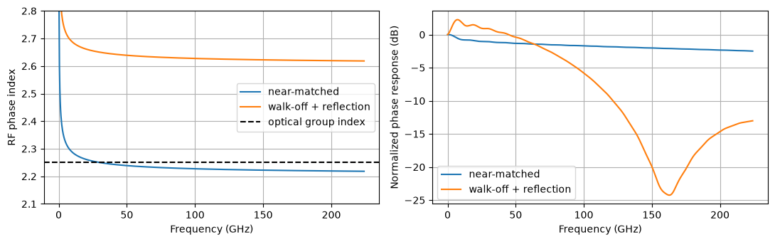
The near-matched design has a 50 Ω source/load. A second design adds walk-off and a 30 Ω load. These are example parameters, not a fitted TFLN device.
r_dc, z_line = 300.0, 45.0  # ohm/m, ohm
r_skin = 2 * z_line * (0.5e2 * np.log(10) / 20) / np.sqrt(1e9)  # ~0.5 dB/cm at 1 GHz, growing as sqrt(f)


def electrode_rlgc(n_rf):
    """Per-metre R, L, G, C versus Hz; the skin-effect internal inductance keeps the data causal."""

    def r(f):
        return r_dc + r_skin * np.sqrt(f)

    def inductance(f):
        return z_line * n_rf / c0 + np.divide(r_skin * np.sqrt(f), 2 * np.pi * f, out=np.zeros_like(f), where=f > 0)

    def c(f):
        return np.full_like(f, n_rf / (z_line * c0))

    return {"R": r, "L": inductance, "G": 0.0, "C": c}


designs = {
    "near-matched": {"n_rf": 2.2, "load_r": 50.0},
    "walk-off + reflection": {"n_rf": 2.6, "load_r": 30.0},
}
source_r = 50.0
2. Calculate the whole-device reference¤
Light leaving at time \(t\) passed position \(z\) at \(t-\tau(z)\), where \(\tau(z)=(L-z)n_{g,\mathrm{opt}}/c\). With the \(e^{j\omega t}\) convention, the path-averaged voltage response is
Here \(V_s\) is the open-circuit source voltage; \(V(z,f)\) includes RF loss, walk-off and source/load reflections. section_veff evaluates this integral for a uniform line in closed form. \(H_V\) has units V/V and is not the electrode's electrical \(S_{21}\).
For a linear Pockels law \(\Delta n=aV\), the push-pull differential-phase response and phase waveform are
phase_transfer returns \(H_\phi\) in rad/V. time_response implements this convolution by FFT multiplication. The circuit comparison reuses this single reference. For measured data, supply a calibrated complex phase response with the same source/load convention; converting a detected-power response requires the optical bias slope and receiver de-embedding.
Uniform-line treatment: H. Chung, W. S. C. Chang and E. L. Adler, “Modeling and optimization of traveling-wave LiNbO₃ interferometric modulators,” IEEE Journal of Quantum Electronics 27(3), 608–617 (1991). The normalized phase-response magnitude is plotted below.
def propagation(f, n_rf):
    """Propagation constant (1/m) and characteristic impedance (ohm)."""
    rlgc = electrode_rlgc(n_rf)
    f = np.maximum(np.asarray(f, dtype=float), 1e3)  # zero-frequency voltages use their exact DC limits below
    s = 2j * np.pi * f
    z, y = rlgc["R"](f) + s * rlgc["L"](f), s * rlgc["C"](f)
    return np.sqrt(z * y), np.sqrt(z / y)


def electrode_voltage(f, positions, *, n_rf, load_r):
    """Local electrode voltage per open-circuit source volt; shape (positions, frequencies)."""
    f, z = np.asarray(f, dtype=float), np.asarray(positions)[:, None]
    gamma, zc = propagation(f, n_rf)
    ch, sh = np.cosh(gamma * length_m), np.sinh(gamma * length_m)
    v_load = 1 / (ch + zc * sh / load_r + source_r * (sh / zc + ch / load_r))
    distance = length_m - z
    voltage = v_load * (np.cosh(gamma * distance) + zc / load_r * np.sinh(gamma * distance))
    dc = (load_r + r_dc * distance) / (source_r + load_r + r_dc * length_m)
    return np.where(f == 0, dc, voltage)


def section_veff(f, edges, **design):
    """Mean voltage in each section, delayed to the optical output, per source volt."""
    f = np.asarray(f, dtype=float)
    gamma, _ = propagation(f, design["n_rf"])
    k = 2j * np.pi * f * n_opt / c0
    voltage = electrode_voltage(f, edges, **design)
    out = []
    for i, (za, zb) in enumerate(pairwise(edges)):
        distance = zb - za
        e = np.exp(-gamma * distance)
        co = np.exp(-k * distance) * -np.expm1(-(gamma - k) * distance) / ((gamma - k) * distance)
        counter = -np.expm1(-(gamma + k) * distance) / ((gamma + k) * distance)
        h1, h2 = (co - e * counter) / (1 - e**2), (counter - e * co) / (1 - e**2)
        effective = (h1 * voltage[i] + h2 * voltage[i + 1]) * np.exp(-k * (length_m - zb))
        out.append(np.where(f == 0, (voltage[i] + voltage[i + 1]) / 2, effective))
    return np.asarray(out)


def phase_transfer(f, **design):
    """Whole-device differential phase per open-circuit source volt, in rad/V."""
    return 2 * phase_per_index * dn_dv * section_veff(f, [0.0, length_m], **design)[0]


def time_response(transfer, drive_t, drive_v, output_times, *, dt, guard_records=4):
    """Filter the PWL drive by FFT; constant guard intervals suppress circular wrap-around."""
    record = output_times[-1]
    t = np.arange(-guard_records * record, (guard_records + 1) * record, dt)
    v = np.interp(t, drive_t, drive_v)  # hold the first/last PWL values outside the drive record
    f = np.fft.rfftfreq(len(t), dt)
    response = np.fft.irfft(np.fft.rfft(v) * np.atleast_2d(transfer(f)), len(t), axis=-1)
    return np.asarray([np.interp(output_times, t, row) for row in response])


f_plot = np.linspace(0.0, 2 * baud, 801)
fig, axes = plt.subplots(1, 2, figsize=(11, 3.5))
for name, design in designs.items():
    h_voltage = section_veff(f_plot, [0.0, length_m], **design)[0]
    n_phase = c0 * propagation(f_plot[1:], design["n_rf"])[0].imag / (2 * np.pi * f_plot[1:])
    axes[0].plot(f_plot[1:] / 1e9, n_phase, label=name)
    axes[1].plot(f_plot / 1e9, 20 * np.log10(np.abs(h_voltage / h_voltage[0])), label=name)
axes[0].axhline(n_opt, color="k", linestyle="--", label="optical group index")
axes[0].set(xlabel="Frequency (GHz)", ylabel="RF phase index", ylim=(2.1, 2.8))
axes[1].set(xlabel="Frequency (GHz)", ylabel="Normalized phase response (dB)")
for ax in axes:
    ax.legend()
plt.tight_layout()
plt.show()
3. Set the drive and optical bias¤
The source swing is the open-circuit Thevenin voltage, before the 50 Ω source resistor. Calibrate it for 4 dB static ER in the near-matched design, then Gaussian-filter a PRBS7 waveform with a −3 dB bandwidth of 0.75 times the baud rate (84 GHz here).
After phase accumulation, apply the full interference law at the selected output port:
This optical transfer remains nonlinear even though voltage-to-phase conversion is linear.
def prbs7_bits(preamble_bits):
    state, pattern = 0x7F, []
    for _ in range(127):
        pattern.append(state & 1)
        state = (state >> 1) | (((state ^ (state >> 1)) & 1) << 6)
    return np.r_[np.full(preamble_bits, pattern[0]), pattern]


def band_limited_drive(bits, vpp, *, bandwidth=drive_bandwidth, points_per_ui=16):
    """Gaussian-filtered NRZ, returned as PWL knots; bandwidth is the amplitude −3 dB point."""
    oversampling = 16
    dt = ui / (oversampling * points_per_ui)
    nrz = vpp * (np.repeat(bits, oversampling * points_per_ui) - 0.5)
    sigma_t = np.sqrt(np.log(2)) / (2 * np.pi * bandwidth)
    smooth = gaussian_filter1d(nrz, sigma=sigma_t / dt, mode="nearest", truncate=8)
    return np.arange(0, len(nrz), oversampling) * dt, smooth[::oversampling]


def mzm_power(delta_theta):
    """Output power / input power at the selected coupler port."""
    return (1 - np.cos(quadrature_phase + delta_theta)) / 2


def fold_eye(times, signal, *, flight_time):
    """Two UI with the same time origin for every model; omit the preamble and endpoints."""
    n_bits = round(times[-1] / ui)
    eye_ui = np.arange(2 * samples_per_ui + 1) / samples_per_ui
    fold_bits = np.arange(preamble_bits + 8, n_bits - 5)
    query = flight_time + (fold_bits[:, None] + 0.5 + eye_ui[None, :]) * ui
    return eye_ui, np.interp(query.ravel(), times, signal).reshape(query.shape)


def plot_eye_density(ax, eye_ui, traces, *, ylim):
    """Bin folded samples into one image; colour is the fraction of traces per bin."""
    # The final point duplicates the start of the next two-UI window.
    values = np.asarray(traces)[:, :-1]
    counts, _, _ = np.histogram2d(
        np.broadcast_to(eye_ui[:-1], values.shape).ravel(),
        values.ravel(),
        bins=(eye_ui, np.linspace(*ylim, 161)),
    )
    density = counts.T / len(traces)
    ax.set_facecolor("black")
    ax.grid(False)
    return ax.imshow(
        np.ma.masked_equal(density, 0),
        origin="lower",
        extent=(eye_ui[0], eye_ui[-1], *ylim),
        aspect="auto",
        interpolation="nearest",
        cmap="magma",
        norm=LogNorm(vmin=1 / max(2, len(traces)), vmax=1),
    )


bits = prbs7_bits(preamble_bits)[: preamble_bits + data_bits]
times = np.arange(len(bits) * samples_per_ui + 1) * ui / samples_per_ui
analysis_window = (times >= (preamble_bits + 8) * ui) & (times < (len(bits) - 5) * ui)
design = designs["near-matched"]
dc_gain = section_veff([0.0], [0.0, length_m], **design)[0, 0].real
power_ratio = 10 ** (target_er_db / 10)
contrast = (power_ratio - 1) / (power_ratio + 1)
vpp = np.arcsin(contrast) / (phase_per_index * dn_dv * dc_gain)
drive_t, drive_v = band_limited_drive(bits, vpp)
fft_dt = ui / 256
print(f"Record: {preamble_bits} preamble + {data_bits} data UI")
print(f"Source: {vpp:.2f} Vpp; static effective voltage: ±{dc_gain * vpp / 2:.3f} V")
print(f"Drive: {baud / 1e9:.0f} Gbaud; Gaussian -3 dB bandwidth: {drive_bandwidth / 1e9:.0f} GHz")
Record: 16 preamble + 127 data UI
Source: 2.93 Vpp; static effective voltage: ±0.732 V
Drive: 112 Gbaud; Gaussian -3 dB bandwidth: 84 GHz
4. Build the Circulax model¤
A source-to-phase response folds the electrode and its terminations into one block. A circuit simulator instead needs port currents and voltages: driver impedance, reflections and loading are solved together, including when connected components are nonlinear. The same RF two-port can be reused with different drivers and loads; the end-to-end response then follows from the circuit.
We keep sections to expose local optical coupling and distributed loading. Dynamical states summarize RF memory, while explicit delays use bounded history. This fits incremental transient solving; an offline FFT calculation assumes the input waveform is already known.
Each 250 µm optical section senses an electrode midpoint. phase_shifter_factory(..., junction=None) adds no electrical loading: electrode capacitance is already in RLGC. The arms have opposite Pockels signs, equal transit times and a fixed quadrature offset.
Fit one 125 µm RF half-section through six driver bandwidths and reuse it. characteristic_rlgc_transmission_line uses dynamical states plus explicit delay, checking stability and sampled passivity. For a passive RLC ladder, see rlgc_transmission_line. Neither method certifies arbitrary input data as causal.
Midpoint sampling, RF fitting and transient time stepping contribute separate errors.
design = designs["near-matched"]
section_um = 250.0
half_section = characteristic_rlgc_transmission_line(
    np.r_[0.0, np.geomspace(1e5, 6 * drive_bandwidth, 400)], **electrode_rlgc(design["n_rf"]), length=section_um * 0.5e-6
)
PockelsSection = phase_shifter_factory(delta_neff=linear_index, junction=None, name="PockelsSection")


def sectioned_mzm(drive_t, drive_v, *, design, section_um, line_model):
    """Source -> sectioned electrode -> load; each arm senses the same midpoint taps."""
    n_sections = round(length_m * 1e6 / section_um)
    ins = {
        "GND": {"component": "ground"},
        "VS": {"component": "drive", "settings": {"kind": WAVE_PWL, "pwl_t": jnp.asarray(drive_t), "pwl_v": jnp.asarray(drive_v)}},
        "RS": {"component": "R", "settings": {"R": source_r}},
        "RL": {"component": "R", "settings": {"R": design["load_r"]}},
        "LASER": {"component": "laser", "settings": {"power": 1.0}},
        "SPLIT": {"component": "coupler", "settings": {"coupling": 0.5}},
        "COMBINE": {"component": "coupler", "settings": {"coupling": 0.5}},
        # Carrier phase only: equal arm transit times are supplied by the phase-shifter chain.
        "BIAS": {
            "component": "bias",
            "settings": {
                "length_um": 1.0,
                "neff": -quadrature_phase * wavelength_nm / (2 * np.pi * 1e3),
                "loss_dB_cm": 0.0,
                "center_wavelength_nm": wavelength_nm,
                "wavelength_nm": wavelength_nm,
            },
        },
    }
    con = {"VS,p1": "RS,p1", "VS,p2": "GND,p1", "RL,p2": "GND,p1", "LASER,p1": "SPLIT,p1", "LASER,p2": "GND,p1"}
    for dump in ("DUMP_IN", "DUMP_OUT", "LOAD"):
        ins[dump] = {"component": "R", "settings": {"R": 1.0}}
        con[f"{dump},p2"] = "GND,p1"
    con.update({"SPLIT,p2": "DUMP_IN,p1", "COMBINE,p4": "DUMP_OUT,p1", "COMBINE,p3": "LOAD,p1", "BIAS,p2": "COMBINE,p2"})
    node = "RS,p2"
    for k in range(n_sections):
        ins[f"E{k}a"], ins[f"E{k}b"] = {"component": "line"}, {"component": "line"}
        con[f"E{k}a,p1"], con[f"E{k}b,p1"] = node, f"E{k}a,p2"
        node = f"E{k}b,p2"
        for arm, sign, start, end in (("A", 1.0, "SPLIT,p3", "COMBINE,p1"), ("B", -1.0, "SPLIT,p4", "BIAS,p1")):
            settings = {"length_um": section_um, "n_group": n_opt, "neff": 1.9, "wavelength_nm": wavelength_nm, "sign": sign}
            ins[f"{arm}{k}"] = {"component": "pockels", "settings": settings}
            con[f"{arm}{k},anode"], con[f"{arm}{k},cathode"] = f"E{k}a,p2", "GND,p1"
            con[f"{arm}{k},o1"] = start if k == 0 else f"{arm}{k - 1},o2"
            if k == n_sections - 1:
                con[f"{arm}{k},o2"] = end
    con[node] = "RL,p1"
    net = {"instances": ins, "connections": con, "ports": {"output": "LOAD,p1"}}
    models = {
        "drive": WaveformVoltageSource,
        "R": Resistor,
        "line": line_model,
        "pockels": PockelsSection,
        "laser": OpticalSource,
        "coupler": DirectionalCoupler,
        "bias": OpticalWaveguide,
    }
    return compile_circuit(net, models, is_complex=True, rtol=1e-9, atol=1e-10)


mzm = sectioned_mzm(drive_t, drive_v, design=design, section_um=section_um, line_model=half_section)
5. Run and check the eye¤
Compare the sectioned Circulax circuit with one whole-device convolution reference: filter the same PWL source into differential phase, then apply the full MZM interference law. The closed-form case makes numerical error measurable.
Errors use the settled record without shifting either waveform; the eyes share one flight-time offset. Circuit error includes midpoint sampling, RF fitting, time integration and delay interpolation. Use section length, RF-fit tolerance and time step to check the accuracy required. The residual measures these numerical approximations in this verification case.
solution = mzm.transient(
    t0=0.0,
    t1=float(times[-1]),
    dt0=ui / 128,
    saveat=SaveAt(ts=jnp.asarray(times), fn=lambda t, y, args: mzm.port(y, "output")),
    max_steps=130 * len(bits) + 100,
    throw=True,
)
# Save only the optical output; internal states remain in the solver and delay history.
sectioned_power = np.abs(np.asarray(solution.ys)) ** 2

# Independent reference: whole-device phase convolution, then optical interference.
reference_phase = time_response(lambda f: phase_transfer(f, **design), drive_t, drive_v, times, dt=fft_dt)[0]
closed_power = mzm_power(reference_phase)


def power_errors(power, reference=closed_power):
    """Absolute fractions of input optical power, on the shared settled window."""
    error = (power - reference)[analysis_window]
    return np.sqrt(np.mean(error**2)), np.max(np.abs(error))


rms, maximum = power_errors(sectioned_power)
print(f"Circulax vs convolution reference: RMS {rms:.2e}, max |difference| {maximum:.2e} (fraction of input power)")
assert np.all(np.isfinite(sectioned_power))
assert np.min(sectioned_power) >= 0
assert np.max(sectioned_power) <= 1.001
assert rms < 1e-3

fig, axes = plt.subplots(1, 3, figsize=(15, 4), layout="constrained")
flight_time = length_m * n_opt / c0
for ax, label, power in (
    (axes[0], "Whole-device convolution reference", closed_power),
    (axes[1], "Circulax circuit", sectioned_power),
):
    eye_ui, eye = fold_eye(times, power, flight_time=flight_time)
    image = plot_eye_density(ax, eye_ui, eye, ylim=(0.0, 1.0))
    ax.set(xlabel="Time (UI)", ylabel="Output power / input power", title=label, xlim=(0, 2))
fig.colorbar(image, ax=list(axes[:2]), label="Fraction of traces")
fig.suptitle(f"{baud / 1e9:.0f} Gbaud eye density comparison")
view = (times >= (preamble_bits + 12) * ui) & (times <= (preamble_bits + 20) * ui)
axes[2].plot(times[view] / ui, (sectioned_power - closed_power)[view], color="C2")
axes[2].axhline(0.0, color="k", linestyle=":", lw=0.8)
axes[2].set(
    xlabel="Time (UI, unshifted)", ylabel="(Circulax - reference) / input power", title="Circuit error relative to convolution"
)
plt.show()
E1111 10:39:30.648541    7247 slow_operation_alarm.cc:73] Constant folding an instruction is taking > 1s:

  %sort.4 = (s32[77216]{0}, s32[77216]{0}, s64[77216]{0}) sort(%constant.631, %constant.630, %iota.195), dimensions={0}, is_stable=true, to_apply=%region_36.66, metadata={op_name="jit(fixed_point)/while/body/jit(_solve_with_symbol_jit)/jit(lexsort)/sort" source_file="/home/runner/work/circulax/circulax/circulax/solvers/linear.py" source_line=510 source_end_line=516 source_column=19 source_end_column=9}

This isn't necessarily a bug; constant-folding is inherently a trade-off between compilation time and speed at runtime. XLA has some guards that attempt to keep constant folding from taking too long, but fundamentally you'll always be able to come up with an input program that takes a long time.

If you'd like to file a bug, run with envvar XLA_FLAGS=--xla_dump_to=/tmp/foo and attach the results.


E1111 10:39:31.799007    7150 slow_operation_alarm.cc:140] The operation took 2.150561297s
Constant folding an instruction is taking > 1s:

  %sort.4 = (s32[77216]{0}, s32[77216]{0}, s64[77216]{0}) sort(%constant.631, %constant.630, %iota.195), dimensions={0}, is_stable=true, to_apply=%region_36.66, metadata={op_name="jit(fixed_point)/while/body/jit(_solve_with_symbol_jit)/jit(lexsort)/sort" source_file="/home/runner/work/circulax/circulax/circulax/solvers/linear.py" source_line=510 source_end_line=516 source_column=19 source_end_column=9}

This isn't necessarily a bug; constant-folding is inherently a trade-off between compilation time and speed at runtime. XLA has some guards that attempt to keep constant folding from taking too long, but fundamentally you'll always be able to come up with an input program that takes a long time.

If you'd like to file a bug, run with envvar XLA_FLAGS=--xla_dump_to=/tmp/foo and attach the results.


Circulax vs convolution reference: RMS 2.23e-04, max |difference| 6.02e-04 (fraction of input power)
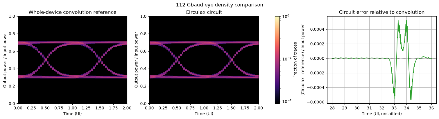
The agreement checks the circuit realization against the uniform-line limit. Phase convolution remains a useful shortcut for a standalone device with fixed terminations. Circulax retains the electrical ports and local optical coupling needed to connect drivers, bias networks and distributed loads, without first deriving a new end-to-end transfer function.