Propagation delay and cable loss¤

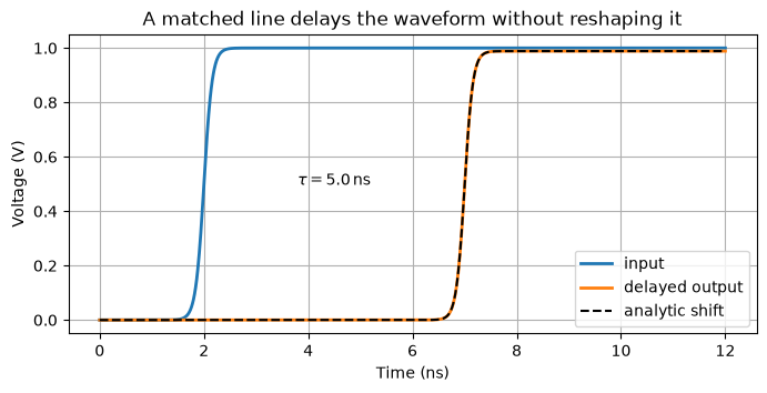
First we check TransmissionLine as a simple delay reference in transient, AC, and harmonic balance:

\[b_1(t)=a\,a_2(t-\tau), \qquad b_2(t)=a\,a_1(t-\tau).\]

This primitive applies a fixed delay and constant attenuation. It does not model skin effect. The reference uses a 5 ns delay and just 0.1 dB loss.

The noisy cable example then adds frequency-dependent conductor loss and its associated dispersion, extending to 40 GHz. We fit that response with a rational core and explicit propagation delays, then compare the fitted pulse with an independent time-domain calculation.

import jax
import jax.numpy as jnp
import matplotlib.pyplot as plt
import numpy as np

from circulax import compile_circuit
from circulax.components.electronic import Resistor, SmoothPulse, TransmissionLine, VoltageSourceAC

jax.config.update("jax_enable_x64", True)
plt.rcParams.update({"figure.figsize": (8, 3.5), "axes.grid": True})

Transient: watch the edge move¤

A smooth step drives a matched line. Because the load equals \(Z_0\), there is no reflection and the output should be an attenuated copy of the input shifted by \(\tau\). Constant DC prehistory means no artificial edge appears at startup.

tau = 5.0e-9
z0 = 50.0
insertion_loss_db = 0.1
attenuation = 10 ** (-insertion_loss_db / 20)
source_delay = 2.0e-9
rise_time = 0.8e-9

models = {
    "source": SmoothPulse,
    "line": TransmissionLine,
    "resistor": Resistor,
    "ground": lambda: 0,
}

transient_netlist = {
    "instances": {
        "GND": {"component": "ground"},
        "VIN": {
            "component": "source",
            "settings": {"V": 1.0, "delay": source_delay, "tr": rise_time},
        },
        "TL": {
            "component": "line",
            "settings": {"tau": tau, "z0": z0, "attenuation": attenuation},
        },
        "RL": {"component": "resistor", "settings": {"R": z0}},
    },
    "connections": {
        "GND,p1": ("VIN,p2", "RL,p2"),
        "VIN,p1": "TL,p1",
        "TL,p2": "RL,p1",
    },
    "ports": {"input": "TL,p1", "output": "TL,p2"},
}

transient_circuit = compile_circuit(transient_netlist, models)

sample_times = jnp.linspace(0.0, 12.0e-9, 1201)
solution = transient_circuit.transient(
    t0=0.0,
    t1=float(sample_times[-1]),
    dt0=1.0e-11,
    saveat=sample_times,
    max_steps=4000,
    throw=True,
)

v_in = transient_circuit.port(solution.ys, "input")
v_out = transient_circuit.port(solution.ys, "output")
analytic_out = attenuation * jax.nn.sigmoid(
    10.0 * (sample_times - source_delay - tau) / rise_time
)
max_transient_error = float(jnp.max(jnp.abs(v_out - analytic_out)))
print(f"Maximum transient error: {max_transient_error:.2e}")
assert max_transient_error < 2e-4

Maximum transient error: 4.01e-11

fig, ax = plt.subplots()
ax.plot(sample_times * 1e9, v_in, label="input", lw=2)
ax.plot(sample_times * 1e9, v_out, label="delayed output", lw=2)
ax.plot(sample_times * 1e9, analytic_out, "k--", label="analytic shift", lw=1.5)
ax.annotate(
    rf"$\tau={tau * 1e9:.1f}\,\mathrm{{ns}}$",
    xy=(source_delay * 1e9 + tau * 1e9 / 2, attenuation / 2),
    ha="center",
)
ax.set(xlabel="Time (ns)", ylabel="Voltage (V)", title="A matched line delays the waveform without reshaping it")
ax.legend()
plt.show()

AC: read the same delay from phase¤

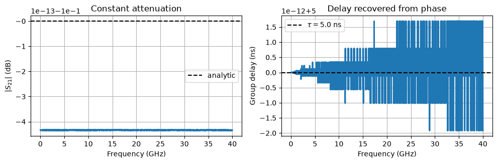
For a matched line, \(S_{21}=a\exp(-j2\pi f\tau)\). Its magnitude is constant and its unwrapped phase is linear, so the group delay is

\[-\frac{1}{2\pi}\frac{d\angle S_{21}}{df}=\tau.\]

# Very large shunts register both external nodes while changing S by less than 1e-11.
ac_netlist = {
    "instances": {
        "GND": {"component": "ground"},
        "TL": {
            "component": "line",
            "settings": {"tau": tau, "z0": z0, "attenuation": attenuation},
        },
        "R1": {"component": "resistor", "settings": {"R": 1e15}},
        "R2": {"component": "resistor", "settings": {"R": 1e15}},
    },
    "connections": {
        "GND,p1": ("R1,p2", "R2,p2"),
        "TL,p1": "R1,p1",
        "TL,p2": "R2,p1",
    },
    "ports": {"port1": "TL,p1", "port2": "TL,p2"},
}

ac_circuit = compile_circuit(ac_netlist, models)
frequencies = jnp.asarray(np.linspace(1e6, 40e9, 4001))
scattering = ac_circuit.sp(ports=["port1", "port2"], freqs=frequencies, z0=z0)
s21 = scattering[:, 1, 0]
analytic_s21 = attenuation * jnp.exp(-2j * jnp.pi * frequencies * tau)
max_ac_error = float(jnp.max(jnp.abs(s21 - analytic_s21)))
print(f"Maximum AC error: {max_ac_error:.2e}")
assert max_ac_error < 1e-9

Maximum AC error: 4.96e-14

phase = np.unwrap(np.angle(np.asarray(s21)))
group_delay = -np.gradient(phase, np.asarray(frequencies)) / (2 * np.pi)

fig, (ax_mag, ax_delay) = plt.subplots(1, 2, figsize=(10, 3.5))
ax_mag.plot(np.asarray(frequencies) / 1e9, 20 * np.log10(np.abs(np.asarray(s21))), lw=2)
ax_mag.axhline(20 * np.log10(attenuation), color="k", ls="--", label="analytic")
ax_mag.set(xlabel="Frequency (GHz)", ylabel=r"$|S_{21}|$ (dB)", title="Constant attenuation")
ax_mag.legend()

ax_delay.plot(np.asarray(frequencies) / 1e9, group_delay * 1e9, lw=2)
ax_delay.axhline(tau * 1e9, color="k", ls="--", label=rf"$\tau={tau * 1e9:.1f}$ ns")
ax_delay.set(xlabel="Frequency (GHz)", ylabel="Group delay (ns)", title="Delay recovered from phase")
ax_delay.legend()
plt.tight_layout()
plt.show()

Harmonic balance: rotate each harmonic¤

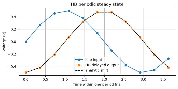
HB represents a periodic waveform by harmonics of a fundamental frequency \(f_0\). The solver applies the delay to harmonic \(k\) as

\[X_k(t-\tau)=X_k(t)\exp(-j2\pi kf_0\tau).\]

Here a sinusoidal source drives the same matched line through a \(50\,\Omega\) source resistance. We compare the fundamental output/input ratio with the same analytical factor used for AC.

fundamental = 250e6
hb_netlist = {
    "instances": {
        "GND": {"component": "ground"},
        "VS": {"component": "source_ac", "settings": {"V": 1.0, "freq": fundamental}},
        "RS": {"component": "resistor", "settings": {"R": z0}},
        "TL": {
            "component": "line",
            "settings": {"tau": tau, "z0": z0, "attenuation": attenuation},
        },
        "RL": {"component": "resistor", "settings": {"R": z0}},
    },
    "connections": {
        "GND,p1": ("VS,p2", "RL,p2"),
        "VS,p1": "RS,p1",
        "RS,p2": "TL,p1",
        "TL,p2": "RL,p1",
    },
    "ports": {"line_input": "TL,p1", "line_output": "TL,p2"},
}

hb_models = {**models, "source_ac": VoltageSourceAC}
hb_circuit = compile_circuit(hb_netlist, hb_models, backend="dense")
hb_time, hb_spectrum = hb_circuit.hb(
    freq=fundamental,
    harmonics=5,
    rtol=1e-9,
    atol=1e-9,
    max_steps=30,
)

input_spectrum = hb_circuit.port(hb_spectrum, "line_input")
output_spectrum = hb_circuit.port(hb_spectrum, "line_output")
hb_ratio = output_spectrum[1] / input_spectrum[1]
analytic_ratio = attenuation * jnp.exp(-2j * jnp.pi * fundamental * tau)
hb_error = float(jnp.abs(hb_ratio - analytic_ratio))
higher_harmonics = float(jnp.max(jnp.abs(output_spectrum[2:])))

print(f"HB fundamental ratio: {hb_ratio:.6f}")
print(f"Analytical ratio:      {analytic_ratio:.6f}")
print(f"Fundamental error:     {hb_error:.2e}")
print(f"Largest higher harmonic: {higher_harmonics:.2e}")
assert hb_error < 2e-7
assert higher_harmonics < 2e-8

HB fundamental ratio: -0.000000-0.988553j
Analytical ratio:      0.000000-0.988553j
Fundamental error:     2.78e-11
Largest higher harmonic: 6.53e-17

hb_times = np.arange(hb_time.shape[0]) / (hb_time.shape[0] * fundamental)
hb_input = np.asarray(hb_circuit.port(hb_time, "line_input"))
hb_output = np.asarray(hb_circuit.port(hb_time, "line_output"))
expected_hb_output = 0.5 * attenuation * np.sin(2 * np.pi * fundamental * (hb_times - tau))

fig, ax = plt.subplots()
ax.plot(hb_times * 1e9, hb_input, "o-", label="line input")
ax.plot(hb_times * 1e9, hb_output, "o-", label="HB delayed output")
ax.plot(hb_times * 1e9, expected_hb_output, "k--", label="analytic shift")
ax.set(xlabel="Time within one period (ns)", ylabel="Voltage (V)", title="HB periodic steady state")
ax.legend()
plt.show()

The reference checks recover the configured 5 ns delay with 0.1 dB constant loss. The fitting API can infer this propagation delay for a passive, approximately reciprocal, low-reflection two-port. It reserves every fifth frequency while comparing the rational-only and delayed candidates, then refits the selected configuration on all samples.

from circulax.fitting import ModelFitOptions, fit_model

inference_frequencies = np.asarray(frequencies)[::4]
inference_s = np.asarray(scattering)[::4]
inferred_fit = fit_model(
    inference_s,
    inference_frequencies,
    z0=z0,
    options=ModelFitOptions(delay_mode="infer", max_delay=6e-9),
)
print(f"Inferred propagation delay: {inferred_fit.port_delays.sum() * 1e9:.3f} ns")
print(inferred_fit.metadata["delay_inference"]["reservation"])
np.testing.assert_allclose(inferred_fit.port_delays.sum(), tau, rtol=1e-4)

Inferred propagation delay: 5.000 ns
{'fraction': 0.2, 'training_samples': 801, 'validation_samples': 200}

The inferred path is deliberately narrower than supplied delays: reflective, active, nonreciprocal, or strongly dispersive data require a physical delay model or supplied per-port delays. We now add frequency-dependent loss and supply the known propagation delay.

Fit a noisy cable response¤

For a known cable, the usual starting point would be a physical transmission-line model fitted to its geometry and material properties. Here we use a simplified matched model to illustrate delay-aware rational fitting. Scikit-rf's transmission-line modeling example explains the propagation-constant representation; its coaxial model includes conductor skin effect.

We use a causal square-root loss term:

\[ S_{21}(s)=S_{12}(s)=A_0\exp(-s\tau-k\sqrt{s}),\qquad S_{11}=S_{22}=0. \]

The square root has positive real part for \(\operatorname{Re}s>0\). At \(s=j2\pi f\), it becomes \((1+j)\sqrt{\pi f}\), so the same term produces both attenuation and phase lag. This avoids changing magnitude while leaving an incompatible phase response.

We set \(\tau=5\) ns, \(A_0=10^{-0.1/20}\), and choose \(k\) to give 12 dB total loss at 40 GHz. Insertion loss is then

\[L(f)=0.1+11.9\sqrt{f/(40\,\mathrm{GHz})}\quad\mathrm{dB}.\]

Loss is about 0.16 dB at 1 MHz, rather than 12 dB everywhere. This is a skin-effect-inspired approximation with fixed 50 Ω impedance; it omits dielectric loss, impedance variation, and the transition from skin effect to DC conductor behavior.

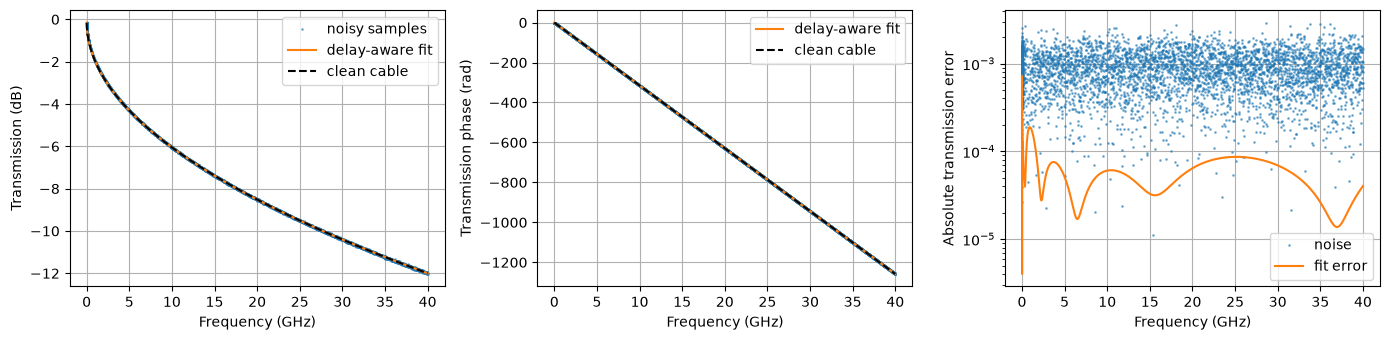
The 4,201-point sweep adds logarithmically spaced samples below 1 GHz to resolve the low-frequency curvature, then uses 10 MHz spacing through 40 GHz. We add complex Gaussian noise with RMS magnitude 0.001 per independent S entry. The transmissions share the same noise to preserve reciprocity; reflection noises are independent. Every fifth sample is held out. A generated Touchstone copy is stored under examples/fitting/data.

This uses per-port de-embedding around conventional vector fitting. The stable fitting workflow is introduced in the vector-fitting tutorial.

from circulax.fitting import ModelCoefficients, ModelFitOptions, circuit_from_coefficients, fit_model, validate_model

fit_frequencies = np.unique(np.r_[np.geomspace(1e6, 1e9, 301), np.linspace(1e9, 40e9, 3901)])
dc_loss_db = 0.1
loss_at_40ghz_db = 12.0
cable_dc_gain = 10 ** (-dc_loss_db / 20)
skin_k = (loss_at_40ghz_db - dc_loss_db) * np.log(10) / (20 * np.sqrt(np.pi * 40e9))


def cable_transfer(freqs):
    s = 2j * np.pi * np.asarray(freqs)
    return cable_dc_gain * np.exp(-s * tau - skin_k * np.sqrt(s))


clean_s = np.zeros((len(fit_frequencies), 2, 2), dtype=complex)
clean_s[:, 0, 1] = clean_s[:, 1, 0] = cable_transfer(fit_frequencies)
clean_loss_db = -20 * np.log10(np.abs(clean_s[:, 1, 0]))
assert np.all(np.diff(clean_loss_db) > 0)
np.testing.assert_allclose(clean_loss_db[[0, -1]], [0.1595, 12.0], atol=1e-10)
assert np.max(np.linalg.svd(clean_s, compute_uv=False)) < 1

noise_rms = 0.001
rng = np.random.default_rng(2026)
noise = noise_rms / np.sqrt(2) * (
    rng.normal(size=(len(fit_frequencies), 3)) + 1j * rng.normal(size=(len(fit_frequencies), 3))
)
noisy_s = clean_s.copy()
noisy_s[:, 0, 0] += noise[:, 0]
noisy_s[:, 0, 1] += noise[:, 1]
noisy_s[:, 1, 0] += noise[:, 1]
noisy_s[:, 1, 1] += noise[:, 2]
train = np.arange(len(fit_frequencies)) % 5 != 0
holdout = ~train
print(f"Training samples: {train.sum()}, held-out samples: {holdout.sum()}")
for f, loss in zip([1e6, 1e9, 10e9, 40e9], -20 * np.log10(np.abs(cable_transfer([1e6, 1e9, 10e9, 40e9]))), strict=True):
    print(f"Loss at {f / 1e9:g} GHz: {loss:.3f} dB")

Training samples: 3360, held-out samples: 841
Loss at 0.001 GHz: 0.160 dB
Loss at 1 GHz: 1.982 dB
Loss at 10 GHz: 6.050 dB
Loss at 40 GHz: 12.000 dB

Fit with the known propagation delay¤

The square-root term adds frequency-dependent group delay. Fitting a straight line to the entire phase would therefore absorb part of the loss dynamics into the delay estimate. The diagnostic below shows the residual from that straight-line fit on training samples.

For this synthetic cable we know the 5 ns travel time and supply it explicitly, splitting it equally between the two port reference planes. The fitter must recover the remaining attenuation and dispersion from noisy samples. We keep the same error targets: 0.8% NRMSE and 0.005 maximum absolute S error.

We also try a rational-only fit with scikit-rf's default automatic-order limit of 100. A failed baseline is reported as such; it doesn't tell us the minimum order of a successful rational-only fit. The largest training frequency gap remains about 20 MHz, which resolves the 5 ns propagation phase.

training_phase = np.unwrap(np.angle(noisy_s[train, 1, 0]))
training_ghz = fit_frequencies[train] / 1e9
phase_line = np.polyfit(training_ghz, training_phase, 1)
phase_residual = np.max(np.abs(training_phase - np.polyval(phase_line, training_ghz)))
print(f"Maximum straight-line phase residual: {phase_residual:.3f} rad")
print(f"Default inferred-delay phase limit: {ModelFitOptions().delay_inference.phase_residual:.3f} rad")

fit_limits = {"normalized_rmse": 0.008, "max_absolute_error": 0.005}
rational_fit = None
try:
    rational_fit = fit_model(
        noisy_s[train], fit_frequencies[train], z0=z0,
        options=ModelFitOptions(delay_mode="none", **fit_limits),
    )
    validate_model(rational_fit, measured_S=noisy_s[train], freqs=fit_frequencies[train]).raise_for_simulation(allow_warnings=True)
except ValueError as error:
    rational_fit = None
    print("Rational-only baseline did not qualify:", error)

delayed_fit = fit_model(
    noisy_s[train], fit_frequencies[train], z0=z0,
    options=ModelFitOptions(delay_mode="supplied", port_delays=(tau / 2, tau / 2), **fit_limits),
)
print(f"Supplied propagation delay: {delayed_fit.port_delays.sum() * 1e9:.3f} ns")
print("Fitted core poles:", len(delayed_fit.poles))
print("Training NRMSE:", delayed_fit.metadata["training_nrmse"])
if rational_fit is not None:
    print("Rational-only poles:", len(rational_fit.poles))
else:
    print("No pole-reduction figure is reported against a failed baseline.")

Maximum straight-line phase residual: 0.302 rad
Default inferred-delay phase limit: 0.050 rad


Rational-only baseline did not qualify: Final fit exceeds accuracy limits: NRMSE=0.725149, max error=0.894528


Supplied propagation delay: 5.000 ns
Fitted core poles: 11
Training NRMSE: 0.0029396270036066933
No pole-reduction figure is reported against a failed baseline.

Check samples the fitter didn't see¤

We compare the accepted fit against the noisy holdout samples and the clean response. A rational-only baseline appears in the table only if it passed the training and realization checks. The clean response is available because this is synthetic data; it isn't used to estimate the delay or choose a fit.

def normalized_error(prediction, reference):
    return np.linalg.norm(prediction - reference) / np.linalg.norm(reference)

print(f"{'Model':<18} {'Poles':>6} {'Holdout NRMSE':>16} {'Holdout max':>14} {'Clean NRMSE':>14}")
comparisons = [("Explicit delays", delayed_fit)]
if rational_fit is not None:
    comparisons.insert(0, ("Rational only", rational_fit))
for label, coefficients in comparisons:
    prediction = coefficients.evaluate(fit_frequencies[holdout])
    measured_error = normalized_error(prediction, noisy_s[holdout])
    maximum = np.max(np.abs(prediction - noisy_s[holdout]))
    clean_error = normalized_error(prediction, clean_s[holdout])
    print(f"{label:<18} {len(coefficients.poles):>6} {measured_error:>16.3e} {maximum:>14.3e} {clean_error:>14.3e}")
    assert measured_error < fit_limits["normalized_rmse"]
    assert maximum < fit_limits["max_absolute_error"]
assert normalized_error(delayed_fit.evaluate(fit_frequencies[holdout]), clean_s[holdout]) < 0.002

fit_s = delayed_fit.evaluate(fit_frequencies)
ghz = fit_frequencies / 1e9
fig, axes = plt.subplots(1, 3, figsize=(14, 3.5))
axes[0].plot(ghz, 20 * np.log10(np.abs(noisy_s[:, 1, 0])), ".", ms=2, alpha=0.5, label="noisy samples")
axes[0].plot(ghz, 20 * np.log10(np.abs(fit_s[:, 1, 0])), label="delay-aware fit")
axes[0].plot(ghz, -clean_loss_db, "k--", label="clean cable")
axes[0].set(xlabel="Frequency (GHz)", ylabel="Transmission (dB)")
axes[0].legend()
axes[1].plot(ghz, np.unwrap(np.angle(noisy_s[:, 1, 0])), ".", ms=2, alpha=0.5)
axes[1].plot(ghz, np.unwrap(np.angle(fit_s[:, 1, 0])), label="delay-aware fit")
axes[1].plot(ghz, np.unwrap(np.angle(clean_s[:, 1, 0])), "k--", label="clean cable")
axes[1].set(xlabel="Frequency (GHz)", ylabel="Transmission phase (rad)")
axes[1].legend()
axes[2].semilogy(ghz, np.abs(noisy_s[:, 1, 0] - clean_s[:, 1, 0]), ".", ms=2, alpha=0.5, label="noise")
axes[2].semilogy(ghz, np.abs(fit_s[:, 1, 0] - clean_s[:, 1, 0]), label="fit error")
axes[2].set(xlabel="Frequency (GHz)", ylabel="Absolute transmission error")
axes[2].legend()
plt.tight_layout()
plt.show()

Model               Poles    Holdout NRMSE    Holdout max    Clean NRMSE
Explicit delays        11        2.928e-03      2.860e-03      1.983e-04

Check pulse spreading in transient¤

The lossy cable's output is no longer a scaled, shifted copy of the input. For the loss factor \(\exp(-k\sqrt{s})\), the normalized step response is

\[g(t)=\operatorname{erfc}\left(\frac{k}{2\sqrt{t}}\right),\quad t>0,\]

and zero before arrival. We integrate this response against the derivative of the smooth input step to get an independent reference waveform. The initial DC value is used as constant prehistory. This calculation uses the analytic cable model, not the fitted poles or a finite-band inverse FFT.

Then we save and reload the coefficients and replace the reference line in the transient circuit with the fitted model. We can check its low-frequency extrapolation against the generating model here; an unknown measured cable would need separate evidence for that extrapolation.

import copy
import tempfile
from pathlib import Path

from scipy.integrate import quad
from scipy.special import erfc, expit

with tempfile.TemporaryDirectory() as directory:
    coefficient_path = Path(directory) / "noisy_line_fit.npz"
    delayed_fit.save(coefficient_path)
    restored_fit = ModelCoefficients.load(coefficient_path)
    fitted_line = circuit_from_coefficients(restored_fit, name="NoisyLineFit")
np.testing.assert_allclose(restored_fit.evaluate(fit_frequencies), fit_s)

fitted_netlist = copy.deepcopy(transient_netlist)
fitted_netlist["instances"]["TL"] = {"component": "fitted_line"}
fitted_circuit = compile_circuit(fitted_netlist, {**models, "fitted_line": fitted_line})
fitted_solution = fitted_circuit.transient(
    t0=0.0, t1=float(sample_times[-1]), dt0=1e-11,
    saveat=sample_times, max_steps=4000, throw=True,
)
fitted_output = np.asarray(fitted_circuit.port(fitted_solution.ys, "output"))
# Convolve the analytic cable step response with the input derivative.
initial_voltage = expit(-10 * source_delay / rise_time)


def cable_pulse_reference(time):
    remaining = float(time) - tau
    if remaining <= 0:
        return cable_dc_gain * initial_voltage

    def integrand(u):
        value = expit(10 * (u - source_delay) / rise_time)
        derivative = 10 / rise_time * value * (1 - value)
        return erfc(skin_k / (2 * np.sqrt(remaining - u))) * derivative

    integral, _ = quad(integrand, 0, remaining, epsabs=1e-10, epsrel=1e-9)
    return cable_dc_gain * (initial_voltage + integral)


cable_reference = np.array([cable_pulse_reference(t) for t in sample_times])
pulse_error = np.max(np.abs(fitted_output - cable_reference))
print(f"Maximum fitted pulse error: {pulse_error:.3e} V")
assert pulse_error < 0.003

fig, (ax_wave, ax_error) = plt.subplots(2, 1, figsize=(8, 5), sharex=True)
ax_wave.plot(sample_times * 1e9, analytic_out, color="0.6", ls=":", label="delay only (0.1 dB)")
ax_wave.plot(sample_times * 1e9, cable_reference, "k--", label="analytic lossy cable")
ax_wave.plot(sample_times * 1e9, fitted_output.real, label="fit from noisy S data")
ax_wave.set(ylabel="Output voltage (V)")
ax_wave.legend()
ax_error.plot(sample_times * 1e9, (fitted_output - cable_reference).real * 1e3)
ax_error.set(xlabel="Time (ns)", ylabel="Error (mV)")
plt.tight_layout()
plt.show()

Maximum fitted pulse error: 8.126e-05 V

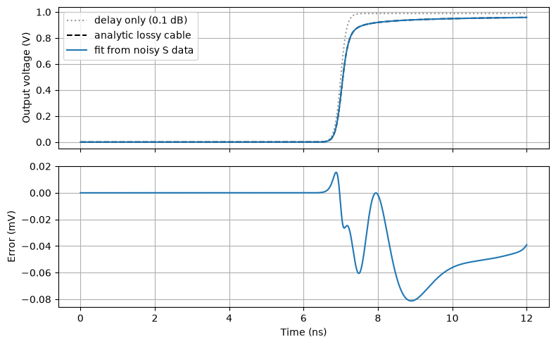
The rational core now represents frequency-dependent attenuation and dispersion. The explicit lines carry the known 5 ns propagation delay. The frequency plot shows low loss at the bottom of the band and 12 dB at 40 GHz; the pulse plot shows the resulting slower edge and settling tail.

The simple phase-linearity assumption used for the previous constant-loss example is no longer appropriate, so this example supplies the propagation delay. It doesn't demonstrate automatic extraction for a dispersive cable. A failed rational-only baseline also doesn't establish the minimum order of a successful higher-order model.

This is a matched, skin-effect-inspired example, not a calibrated model of a particular cable. Dielectric loss, frequency-dependent impedance, and connector reflections would require additional modeling. See the fitting API for fitting and validation options.