A reconfigurable traveling-wave laser¤
A gain section and a passive optical feedback network form a laser cavity. Here every section is a native bidirectional Circulax component: gain cells, optical interfaces, two independently heated sampled Bragg reflectors, and a separate heated phase section. A netlist connects them. Circuit.dc, Circuit.transient, and Circuit.small_signal solve the assembled circuit; there is no separate laser time solver.
left output ↔ sampled Bragg ↔ optical interface ↔ gain cells ↔ optical interface ↔ phase section ↔ sampled Bragg ↔ right output
The outputs have matched terminations. Electrical terminals independently drive the pump and three heaters. We first show seeded startup, then Vernier selection and a wavelength design, and finally replace a grating with a ring-based reflector. Settings are illustrative; the checks establish numerical consistency, not agreement with a fabricated laser. Equations and limitations follow the short worked examples.
import jax
jax.config.update("jax_enable_x64", True)
import jax.numpy as jnp
import matplotlib.pyplot as plt
import numpy as np
from scipy.optimize import minimize
from scipy.integrate import solve_ivp

from circulax import compile_circuit, QuadratureDrive
from circulax.components import (
    HybridSettings, hybrid_laser, hybrid_laser_netlist, ring_reflector,
    MatchedOpticalPulse, TravelingWaveGainCell, SampledBraggGrating,
)
from circulax.components.hybrid_laser import grating_settings, hybrid_threshold, hybrid_modes, hybrid_frame_parameters
from circulax.components.laser_sections import sampled_grating_response
from circulax.components.electronic import Resistor, VoltageSource, WaveformCurrentSource, WAVE_PULSE
from circulax.components.soa import LIGHT_SPEED, ELECTRON_CHARGE, PLANCK
from circulax.components.traveling_wave_laser import (
    LaserParameters, TravelingWaveLaser, traveling_wave_laser, CoherentSeed,
    material_scales, resonant_detuning, seeded_initial_state, threshold,
)
from circulax.components.photonic import OpticalWaveguide
from circulax.components.laser_mirrors import MirrorParameters
from circulax.solvers import BDF2VectorizedTransientSolver, TrapVectorizedTransientSolver

%matplotlib inline
plt.rcParams.update({"figure.figsize": (9, 3.2), "axes.grid": True, "axes.formatter.useoffset": False})
p = LaserParameters()
s = HybridSettings()
# One fixed propagation calibration: the cold reference mode satisfies phase.
g0 = float(hybrid_threshold(p, s, 0., (0., 0., 0.)).gain_m1)
p = p._replace(detuning_rad_s=LIGHT_SPEED / p.group_index * (p.alpha_h * g0 / 2 - np.pi / (2 * p.length_m)))
cold = hybrid_threshold(p, s, 0., (0., 0., 0.))
ith = float(cold.current_a)
M = 4
flight = p.length_m * p.group_index / LIGHT_SPEED
np.testing.assert_allclose(cold.roundtrip, 1., atol=1e-12)
print(f"Cold threshold {ith * 1e3:.4f} mA; active-region one-way flight {flight * 1e12:.4f} ps")
print(f"Grating combs: {s.left_fsr_hz / 1e9:g}, {s.right_fsr_hz / 1e9:g} GHz; {s.samples} patches each")
Cold threshold 59.1087 mA; active-region one-way flight 7.2050 ps
Grating combs: 200, 220 GHz; 5 patches each
Construct and drive the circuit¤
hybrid_laser_netlist returns ordinary editable connectivity and a model map. Gain diodes are in electrical parallel; the optical cells are in series. Each optical interface has 0.5 dB power loss per crossing, and can also represent parasitic reflection. The threshold helper used below assumes reflection-free interfaces. The legacy LaserParameters.r_left/r_right fields are unused here: separate reflector components own reflection and transmission. Heater resistances are 100 Ω, thermal resistances 200 K/W, and thermal time constants 1 µs. A DC solve warms the passive circuit before its much faster optical transient.
hybrid_laser(...) also returns a reusable Circuit subcircuit with exposed optical, pump, and heater ports. Both forms use the same public component equations.
def make_bench(p, s, segments=4, *, right_reflector=None, left_reflector=None, hierarchical=False):
    if hierarchical:
        laser = hybrid_laser(p, s, segments=segments, left_reflector=left_reflector, right_reflector=right_reflector)
        net = {'instances': {'LASER': {'component': 'laser'}}, 'connections': {}, 'ports': {'left': 'LASER,p1', 'right': 'LASER,p2'}}
        models = {'laser': laser}
        ports = {name: f'LASER,{name}' for name in ('p1', 'p2', 'anode', 'cathode', 'heater_left', 'heater_right', 'heater_phase', 'heater_return')}
    else:
        net, models = hybrid_laser_netlist(p, s, segments=segments, left_reflector=left_reflector, right_reflector=right_reflector)
        ports = net['ports'].copy()
        net['ports'] = {'left': ports['p1'], 'right': ports['p2']}
    net['instances'].update({'PUMP': {'component': 'pump'}, 'SEED': {'component': 'seed'}, 'LOAD': {'component': 'load', 'settings': {'R': 1.0}}, 'HL': {'component': 'voltage'}, 'HR': {'component': 'voltage'}, 'HP': {'component': 'voltage'}, 'GND': {'component': 'ground'}})
    net['connections'].update({'GND,p1': (ports['cathode'], ports['heater_return'], 'PUMP,p1', 'SEED,p2', 'LOAD,p2', 'HL,p2', 'HR,p2', 'HP,p2'), 'PUMP,p2': ports['anode'], 'SEED,p1': ports['p1'], 'LOAD,p1': ports['p2'], 'HL,p1': ports['heater_left'], 'HR,p1': ports['heater_right'], 'HP,p1': ports['heater_phase']})
    models.update(pump=WaveformCurrentSource, seed=MatchedOpticalPulse, load=Resistor, voltage=VoltageSource, ground=lambda: 0)
    return compile_circuit(net, models, is_complex=True, backend='klu', g_leak=0, rtol=1e-10, atol=1e-12)

circuit = make_bench(p, s, M)
# Inspect exactly which native sections are connected.
netlist, models = hybrid_laser_netlist(p, s, segments=M)
print({name: row["component"] for name, row in netlist["instances"].items()})


def transient(c, params, *, end=1.5e-9, dt=0.3e-12, save_times=None, initial=None):
    if save_times is None:
        save_times = jnp.linspace(0, end, 501)
    if initial is None:
        initial = c.dc(params=params)
    return c.transient(
        t0=0., t1=end, dt0=dt, y0=initial, saveat=save_times, params=params,
        max_steps=int(np.ceil(end / dt)) + 4, throw=True,
        transient_solver=BDF2VectorizedTransientSolver(linear_solver=c.solver, newton_rtol=1e-9, newton_atol=1e-12),
    )

params = {"PUMP.dc": 1.3 * ith, "SEED.power_w": 1e-12}
startup = transient(circuit, params)
times = np.asarray(startup.ts)
power = np.asarray(abs(circuit.port(startup.ys, "right")) ** 2)
gain = np.stack([np.real(circuit.port(startup.ys, f"GAIN{j},h")) * M / p.length_m for j in range(M)], axis=-1)
density = p.transparency_m3 + gain / (p.confinement * p.differential_gain_m2)
nth = p.transparency_m3 + g0 / (p.confinement * p.differential_gain_m2)
print(f"Final-window right output: {power[-30:].mean() * 1e3:.4f} mW")
{'SG_L': 'grating', 'SG_R': 'grating', 'CHIP_L': 'interface', 'CHIP_R': 'interface', 'PHASE': 'phase', 'GAIN0': 'gain', 'GAIN1': 'gain', 'GAIN2': 'gain', 'GAIN3': 'gain'}


Final-window right output: 2.5156 mW
Seeded startup and carrier clamping¤
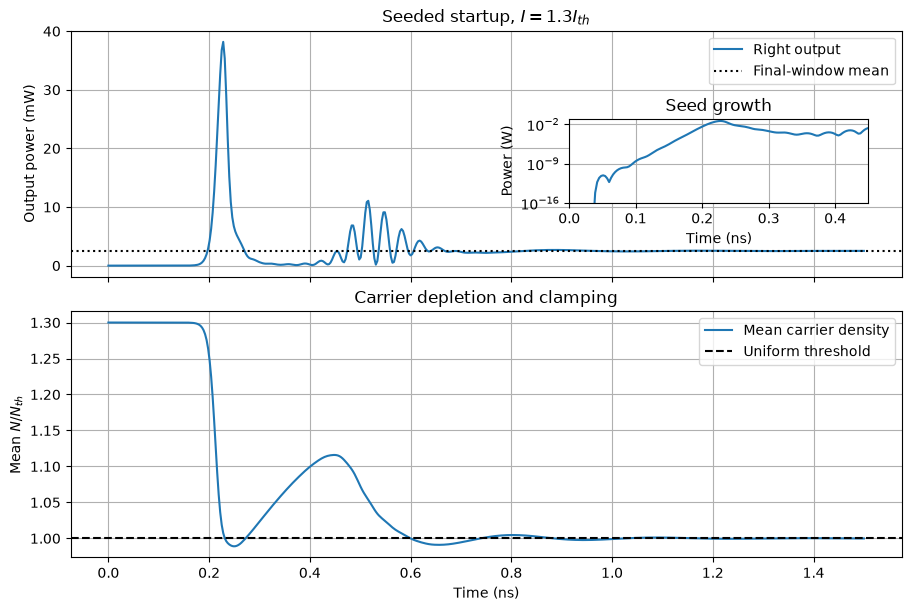
The initial DC state has a pre-biased gain region and exactly zero optical field. A matched source launches a 1 pW peak coherent pulse from 10–40 ps, then absorbs returned light with no further drive. Its field has a sin² envelope; its power has a sin⁴ envelope. This deterministic seed is not spontaneous-emission noise. The initial above-threshold carrier population releases stored energy into the growing field and approaches its lasing value.
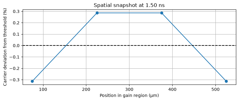
The power plot and carrier plot share the same time axis. The separate spatial snapshot reports small carrier deviations after startup.
fig, axes = plt.subplots(2, 1, figsize=(9, 6), sharex=True, constrained_layout=True)
axes[0].plot(times * 1e9, power * 1e3, label="Right output")
axes[0].axhline(power[-30:].mean() * 1e3, color="k", ls=":", label="Final-window mean")
axes[0].set(ylabel="Output power (mW)", title=r"Seeded startup, $I=1.3 I_{th}$")
axes[0].legend()
inset = axes[0].inset_axes([0.60, 0.30, 0.36, 0.34])
inset.semilogy(times * 1e9, np.maximum(power, 1e-20))
inset.set(xlim=(0, .45), ylim=(1e-16, max(power) * 2), xlabel="Time (ns)", ylabel="Power (W)", title="Seed growth")
axes[1].plot(times * 1e9, density.mean(axis=1) / nth, label="Mean carrier density")
axes[1].axhline(1, color="k", ls="--", label="Uniform threshold")
axes[1].set(xlabel="Time (ns)", ylabel=r"Mean $N/N_{th}$", title="Carrier depletion and clamping")
axes[1].legend()
plt.show()
fig, ax = plt.subplots()
ax.plot((np.arange(M) + .5) * p.length_m / M * 1e6, 100 * (density[-1] / nth - 1), "o-")
ax.axhline(0, color="k", ls="--")
ax.set(xlabel="Position in gain region (µm)", ylabel="Carrier deviation from threshold (%)", title=f"Spatial snapshot at {times[-1] * 1e9:.2f} ns")
plt.show()
Batch native transient solves with JAX¤
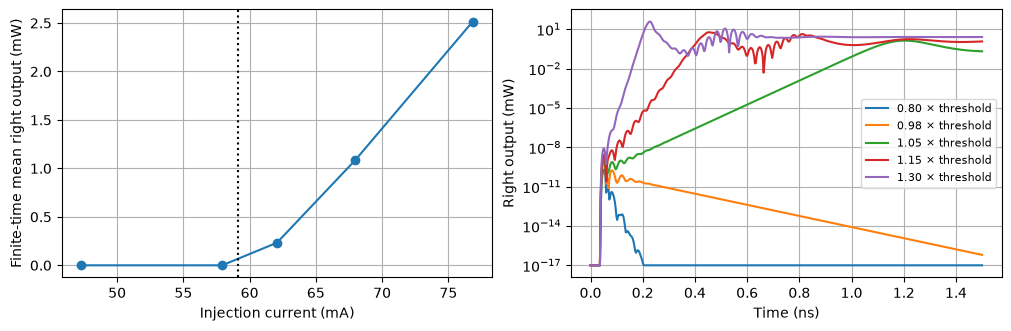
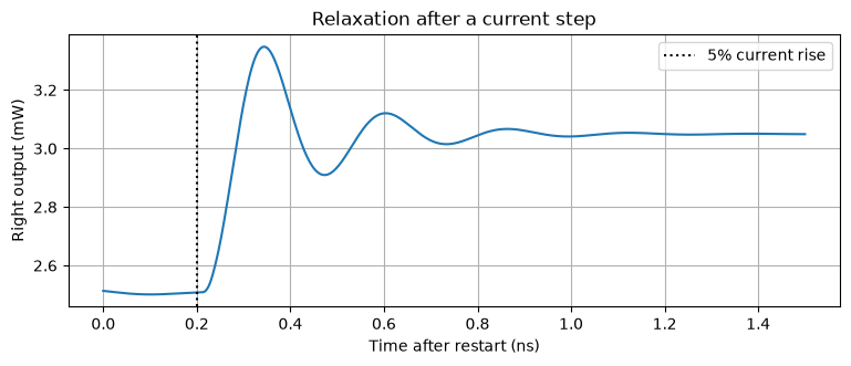
One jax.vmap sweeps injection current through the threshold. The plotted mean is a finite-time mean, not a claim that every point has reached its steady state. Seeded growth slows close to threshold. A second transient then steps the current by 5% to show relaxation.
ratios = jnp.array([.8, .98, 1.05, 1.15, 1.3])

def one_current(ratio):
    sol = transient(circuit, {"PUMP.dc": ratio * ith, "SEED.power_w": 1e-12})
    return abs(circuit.port(sol.ys, "right")) ** 2

batched = jax.jit(jax.vmap(one_current))(ratios)
fig, axes = plt.subplots(1, 2, figsize=(10, 3.2), constrained_layout=True)
axes[0].plot(np.asarray(ratios) * ith * 1e3, np.asarray(batched[:, -30:].mean(axis=1)) * 1e3, "o-")
axes[0].axvline(ith * 1e3, color="k", ls=":")
axes[0].set(xlabel="Injection current (mA)", ylabel="Finite-time mean right output (mW)")
for j in range(len(ratios)):
    axes[1].semilogy(times * 1e9, np.maximum(np.asarray(batched[j]), 1e-20) * 1e3, label=f"{ratios[j]:.2f} × threshold")
axes[1].set(xlabel="Time (ns)", ylabel="Right output (mW)")
axes[1].legend(fontsize=8)
plt.show()

relax = transient(circuit, {"PUMP.dc":1.3*ith, "PUMP.kind":float(WAVE_PULSE), "PUMP.v1":1.3*ith, "PUMP.v2":1.365*ith, "PUMP.delay":.2e-9, "PUMP.tr":20e-12, "PUMP.tf":20e-12, "PUMP.pw":3e-9, "PUMP.per":5e-9, "SEED.power_w":0.}, end=1.5e-9, initial=startup.ys[-1])
fig, ax = plt.subplots()
ax.plot(np.asarray(relax.ts) * 1e9, np.asarray(abs(circuit.port(relax.ys, "right"))**2) * 1e3)
ax.axvline(.2, color="k", ls=":", label="5% current rise")
ax.set(xlabel="Time after restart (ns)", ylabel="Right output (mW)", title="Relaxation after a current step")
ax.legend()
plt.show()
Vary reflector strength¤
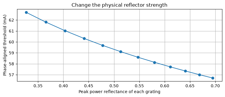
Increasing total Bragg strength changes each reflector's peak power reflectance. Compare the threshold at the reference wavelength while adjusting the independent phase heater to satisfy the cavity phase condition. This parameter sweep uses the same delayed-grating scattering equations as the native components.
strengths = jnp.linspace(.65,1.2,12)

def strength_case(value):
    settings = s._replace(grating_strength=value)
    first = hybrid_threshold(p,settings,0.,(0.,0.,0.))
    phase_temperature = jnp.mod(-jnp.angle(first.roundtrip),2*jnp.pi)/(2*s.phase_per_k)
    aligned = hybrid_threshold(p,settings,0.,(0.,0.,phase_temperature))
    return jnp.tanh(value)**2, aligned.current_a, aligned.roundtrip

reflectance, strength_threshold, roundtrip = jax.jit(jax.vmap(strength_case))(strengths)
np.testing.assert_allclose(roundtrip,1.,atol=1e-12)
fig, ax = plt.subplots()
ax.plot(reflectance,strength_threshold*1e3,"o-")
ax.set(xlabel="Peak power reflectance of each grating",ylabel="Phase-aligned threshold (mA)",title="Change the physical reflector strength")
plt.show()
See the Vernier overlap¤
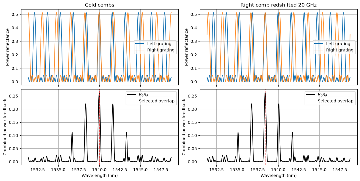
Each sampled reflector produces a reflection comb, with 200 GHz spacing on the left and 220 GHz on the right. Their overlap repeats approximately every $\(F_V=F_LF_R/|F_L-F_R|=2.2\ \mathrm{THz}.\)$ The figure compares the cold combs with a right-grating redshift of 20 GHz. The left comb order at +200 GHz then aligns with the shifted right order at +220−20 GHz. Thus a small redshift of one grating moves the overlap to a shorter laser wavelength. The separate phase section must still align a longitudinal cavity mode there.
These are finite-window reflection and threshold diagnostics. The thin-patch grating approximation repeats indefinitely and omits the finite bandwidth of each physical Bragg patch and of the gain. It cannot establish global wavelength selection or SMSR. The scattering helpers below are exact frequency-domain reductions of the native delayed components, not an alternative transient solver.
target_hz = 200e9
target_wavelength_m = LIGHT_SPEED / (LIGHT_SPEED / p.wavelength_m + target_hz)
right_center_hz = target_hz - s.right_fsr_hz
right_temperature = (LIGHT_SPEED / (LIGHT_SPEED / p.wavelength_m + right_center_hz) - p.wavelength_m) / s.shift_m_per_k
frequencies = jnp.linspace(-1.1e12, 1.1e12, 11001)
wavelengths = LIGHT_SPEED / (LIGHT_SPEED / p.wavelength_m + np.asarray(frequencies)) * 1e9
rl = sampled_grating_response(2*jnp.pi*frequencies, 0., samples=s.samples, **grating_settings(p,s,"left"))[0]
fig, axes = plt.subplots(2, 2, figsize=(12, 6), sharex=True, constrained_layout=True)
for col, temp in enumerate([0., right_temperature]):
    rr = sampled_grating_response(2*jnp.pi*frequencies, temp, samples=s.samples, **grating_settings(p,s,"right"))[0]
    axes[0,col].plot(wavelengths, np.asarray(abs(rl)**2), label="Left grating")
    axes[0,col].plot(wavelengths, np.asarray(abs(rr)**2), label="Right grating", alpha=.85)
    axes[0,col].set(ylabel="Power reflectance", title="Cold combs" if col==0 else "Right comb redshifted 20 GHz")
    axes[0,col].legend()
    axes[1,col].plot(wavelengths, np.asarray(abs(rl*rr)**2), color="black", label=r"$R_L R_R$")
    selected = p.wavelength_m if col==0 else target_wavelength_m
    axes[1,col].axvline(selected*1e9,color="tab:red",ls="--",label="Selected overlap")
    axes[1,col].set(xlabel="Wavelength (nm)", ylabel="Combined power feedback")
    axes[1,col].legend()
plt.show()
print(f"Right grating temperature rise {right_temperature:.4f} K; overlap target {target_wavelength_m*1e9:.6f} nm")
Right grating temperature rise 1.9779 K; overlap target 1538.419463 nm
Explore two independent reflector heaters¤
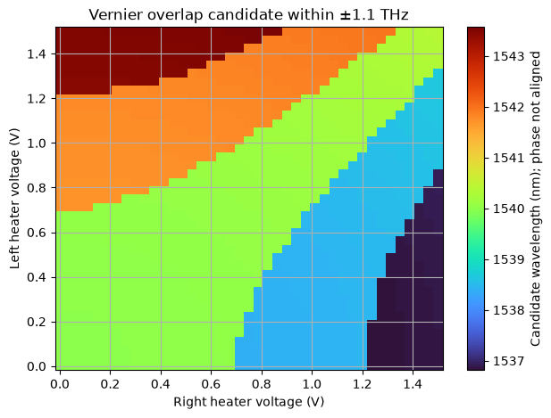
This batched JAX map finds the largest reflector-overlap sample in the stated window. Its branches visualize the Vernier effect. It is a candidate wavelength map: it has no phase constraint and does not simulate laser emission. The next step solves the complete cavity phase and threshold conditions.
voltage_grid = jnp.linspace(0., 1.5, 41)
map_frequencies = jnp.linspace(-1.1e12, 1.1e12, 4401)

def overlap_candidate(vl, vr):
    left = sampled_grating_response(2*jnp.pi*map_frequencies, 2*vl**2, samples=s.samples, **grating_settings(p,s,"left"))[0]
    right = sampled_grating_response(2*jnp.pi*map_frequencies, 2*vr**2, samples=s.samples, **grating_settings(p,s,"right"))[0]
    return map_frequencies[jnp.argmax(abs(left*right)**2)]

candidate_hz = jax.jit(jax.vmap(jax.vmap(overlap_candidate, in_axes=(None,0)), in_axes=(0,None)))(voltage_grid,voltage_grid)
candidate_nm = LIGHT_SPEED / (LIGHT_SPEED/p.wavelength_m + np.asarray(candidate_hz)) * 1e9
fig, ax = plt.subplots(figsize=(7,5))
im = ax.pcolormesh(voltage_grid, voltage_grid, candidate_nm, shading="nearest", cmap="turbo")
ax.set(xlabel="Right heater voltage (V)", ylabel="Left heater voltage (V)", title="Vernier overlap candidate within ±1.1 THz")
fig.colorbar(im, ax=ax, label="Candidate wavelength (nm); phase not aligned")
plt.show()
Design a target wavelength, then verify it in Circulax¤
Optimize three heater voltages for the overlap target. The objective is required threshold current plus a small heater-power penalty, $\(J=I_{th}(\omega_*)/I_{th,0}+10^{-4}\sum_j V_j^2/(1\ \mathrm V)^2.\)$ The equality constraint is zero round-trip phase at the target; we also check the real round-trip field is positive. Temperature states come from native circuit DC solves, and JAX differentiates through those solves and the exact scattering cascade. A centered finite-difference check qualifies the objective and phase derivatives before optimization.
This minimizes target threshold and heating. The competing-mode threshold margin is reported afterward; it is not an SMSR objective. A physical side-mode power ratio requires additional gain-bandwidth/noise physics and a specified spectral measurement.
omega_target = 2*np.pi*target_hz

def conditions(v):
    dc = circuit.dc(params={"PUMP.dc":.8*ith, "SEED.power_w":0., "HL.V":v[0], "HR.V":v[1], "HP.V":v[2]})
    temperatures = tuple(jnp.real(circuit.port(dc,name)) for name in ("SG_L,temperature","SG_R,temperature","PHASE,temperature"))
    return hybrid_threshold(p,s,omega_target,temperatures), temperatures

objective = jax.jit(lambda v: conditions(v)[0].current_a/ith + 1e-4*jnp.sum(v*v))
phase_constraint = jax.jit(lambda v: jnp.angle(conditions(v)[0].roundtrip))
gradient = jax.jit(jax.grad(objective))
phase_gradient = jax.jit(jax.grad(phase_constraint))
phase0 = np.angle(hybrid_threshold(p,s,omega_target,(0.,right_temperature,0.)).roundtrip)
phase_temperature = (-phase0) % (2*np.pi) / (2*s.phase_per_k)
initial_voltages = np.sqrt(np.array([0.,right_temperature,phase_temperature])/2)
trial = initial_voltages + np.array([.1,-.02,.02])
eps = 1e-4
for function, derivative in [(objective,gradient),(phase_constraint,phase_gradient)]:
    fd = np.array([(function(trial+eps*np.eye(3)[j])-function(trial-eps*np.eye(3)[j]))/(2*eps) for j in range(3)])
    np.testing.assert_allclose(derivative(trial),fd,rtol=2e-4,atol=1e-7)
    print("JAX gradient:", np.asarray(derivative(trial)), "finite difference:",fd)
result = minimize(lambda v:float(objective(v)),initial_voltages,jac=lambda v:np.asarray(gradient(v)),method="SLSQP",bounds=[(0.,3.)]*3,constraints={"type":"eq","fun":lambda v:float(phase_constraint(v)),"jac":lambda v:np.asarray(phase_gradient(v))},options={"ftol":1e-12,"maxiter":100})
assert result.success, result.message
voltages = result.x
condition, temperatures = conditions(voltages)
np.testing.assert_allclose(condition.roundtrip,1.,atol=1e-7)
print(f"Target {target_wavelength_m*1e9:.6f} nm; heater voltages L/R/phase = {voltages} V")
print(f"Temperature rises {np.asarray(temperatures)} K; heater power {np.sum(voltages**2)/100*1e3:.4f} mW")
mode_hz, mode_thresholds = hybrid_modes(p,s,temperatures,max_current_a=1.3*ith)
fine_hz, fine_thresholds = hybrid_modes(p,s,temperatures,points=44001,max_current_a=1.3*ith)
np.testing.assert_allclose(mode_hz,fine_hz,atol=1.)
np.testing.assert_allclose(mode_thresholds,fine_thresholds,rtol=1e-9)
order = np.argsort(mode_thresholds)
assert abs(mode_hz[order[0]]-target_hz)<1e8
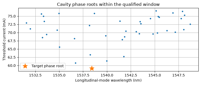
print(f"Target threshold {float(condition.current_a)*1e3:.4f} mA; next-root margin {(mode_thresholds[order[1]]-mode_thresholds[order[0]])*1e3:.4f} mA within ±1.1 THz")
fig, ax = plt.subplots()
ax.plot(LIGHT_SPEED/(LIGHT_SPEED/p.wavelength_m+mode_hz)*1e9,mode_thresholds*1e3,".")
ax.plot(target_wavelength_m*1e9,float(condition.current_a)*1e3,"*",ms=14,label="Target phase root")
ax.set(xlabel="Longitudinal-mode wavelength (nm)",ylabel="Threshold current (mA)",title="Cavity phase roots within the qualified window")
ax.legend()
plt.show()
JAX gradient: [ 0.0001213  -0.00301842  0.00042128] finite difference: [ 0.0001213  -0.00301842  0.00042128]


JAX gradient: [-0.19468061 -1.61782171  2.52770786] finite difference: [-0.19468061 -1.61782173  2.52770786]


Target 1538.419463 nm; heater voltages L/R/phase = [0.         0.99151963 2.08439357] V
Temperature rises [0.         1.96622237 8.68939309] K; heater power 53.2781 mW


Target threshold 59.1087 mA; next-root margin 1.6675 mA within ±1.1 THz
Check the designed branch in a native transient¤
Shift every delayed section into the target envelope frame; the physical cavity calibration stays fixed. The seed then launches the target frequency. Measure the residual envelope phase slope after 5 ns, at both 4 and 8 gain cells. This checks the seeded branch, rather than claiming spontaneous selection from an unspecified noise source.
wavelength_checks = []
for cells in (4,8):
    device = circuit if cells==M else make_bench(p,s,cells)
    updates = {"PUMP.dc":1.15*condition.current_a,"HL.V":voltages[0],"HR.V":voltages[1],"HP.V":voltages[2],"SEED.power_w":1e-12,**hybrid_frame_parameters(omega_target,cells)}
    optical = transient(device,updates,end=5e-9,dt=.2e-12,save_times=jnp.linspace(0,5e-9,1001))
    field = np.asarray(device.port(optical.ys,"right"))
    residual_hz = np.polyfit(np.asarray(optical.ts[-150:]),np.unwrap(np.angle(field[-150:])),1)[0]/(2*np.pi)
    wavelength = LIGHT_SPEED/(LIGHT_SPEED/p.wavelength_m+target_hz+residual_hz)
    wavelength_checks.append(wavelength)
    assert abs(residual_hz)<1e6
    print(f"{cells} cells: {wavelength*1e9:.9f} nm, residual {residual_hz/1e3:.3f} kHz, mean output {np.mean(abs(field[-100:])**2)*1e3:.4f} mW")
assert abs(wavelength_checks[1]-wavelength_checks[0])<1e-13
4 cells: 1538.419462610 nm, residual -2.206 kHz, mean output 1.2533 mW


8 cells: 1538.419462610 nm, residual -2.258 kHz, mean output 1.2533 mW
Replace the feedback technology¤
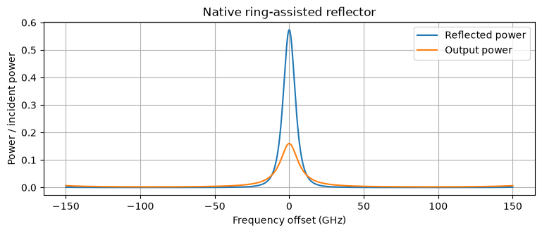
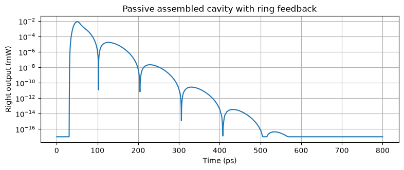
A ring reflector is assembled from two reciprocal directional couplers, two delayed waveguide arms (one heated), a mirror at the drop port, and matched through/add loads. The same optical wave convention supports reverse propagation from that mirror. Its passive spectrum is qualified here, then the actual compiled ring circuit replaces the right Bragg component in a laser subcircuit. A pulse-decay run also exercises the assembled cavity with ring feedback. The public factory accepts left_reflector and right_reflector; replacements use p1 facing the cavity and p2 facing the exterior.
The ring circuit has a different loss, delay, and phase budget. The SG-specific threshold helper and tuned heater solution do not transfer to it. This section demonstrates passive scattering, cavity composition, and passive transient feedback; it does not claim a validated ring-laser operating point. New feedback designs need their own threshold, mode and transient qualification.
def passive_bench(component, settings=None):
    net = {'instances': {'D': {'component': 'device', 'settings': settings or {}}, 'S': {'component': 'source'}, 'LOAD': {'component': 'load', 'settings': {'R': 1.0}}, 'H': {'component': 'voltage'}, 'GND': {'component': 'ground'}}, 'connections': {'S,p1': 'D,p1', 'D,p2': 'LOAD,p1', 'H,p1': 'D,heater', 'GND,p1': ('S,p2', 'LOAD,p2', 'H,p2', 'D,heater_return')}, 'ports': {'out': 'D,p2', 'in': 'D,p1'}}
    return compile_circuit(net, {'device': component, 'source': MatchedOpticalPulse, 'load': Resistor, 'voltage': VoltageSource, 'ground': lambda: 0}, is_complex=True, backend='klu', g_leak=0, rtol=1e-10, atol=1e-12)

replacement = ring_reflector(length_m=400e-6,power_coupling=.2)
ring_bench = passive_bench(replacement)
ring_frequency = jnp.linspace(-150e9,150e9,1001)
response = ring_bench.small_signal(params={"S.power_w":0.})(freqs=ring_frequency,sources={"S":QuadratureDrive(x=1.,y=-1j)})
r = response.sidebands("in")[0]-1. # matched source has a=1, so V=1+b
transmission = response.sidebands("out")[0]
assert np.all(np.asarray(abs(r)**2+abs(transmission)**2)<=1+1e-10)
fig, ax = plt.subplots()
ax.plot(ring_frequency/1e9,abs(r)**2,label="Reflected power")
ax.plot(ring_frequency/1e9,abs(transmission)**2,label="Output power")
ax.set(xlabel="Frequency offset (GHz)",ylabel="Power / incident power",title="Native ring-assisted reflector")
ax.legend()
plt.show()
ring_laser = make_bench(p,s,2,right_reflector=replacement,hierarchical=True)
ring_dc = ring_laser.dc(params={"PUMP.dc":.03,"SEED.power_w":0.,"HR.V":.4})
assert abs(ring_laser.port(ring_dc,"right"))<1e-12
print("Ring feedback connected as a native laser subcircuit; dark electrical DC solved.")


# The same replacement also propagates a pulse in the closed passive cavity.
ring_passive_p = p._replace(transparency_m3=0.,injection_efficiency=0.,saturation=0.,alpha_h=0.,detuning_rad_s=0.)
ring_passive = make_bench(ring_passive_p,s,2,right_reflector=replacement)
ring_pulse = transient(ring_passive,{"PUMP.dc":0.,"SEED.power_w":1e-3},end=.8e-9,dt=.15e-12,save_times=jnp.linspace(0,.8e-9,1601))
ring_power = np.asarray(abs(ring_passive.port(ring_pulse.ys,"right"))**2)
assert ring_power.max()>1e-7
assert ring_power[-100:].max()<ring_power.max()*1e-5
fig, ax = plt.subplots()
ax.semilogy(np.asarray(ring_pulse.ts)*1e12,np.maximum(ring_power,1e-20)*1e3)
ax.set(xlabel="Time (ps)",ylabel="Right output (mW)",title="Passive assembled cavity with ring feedback")
plt.show()
Ring feedback connected as a native laser subcircuit; dark electrical DC solved.
Check numerical resolution and passive timing¤
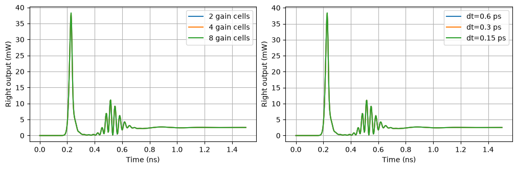
Hold physical grating geometry fixed. Refining the gain cells reduces the arrival-time frozen-gain approximation; changing the number of grating patches changes the physical reflector and is not a mesh-convergence test. Refine the time step separately: several different physical delays are off the integration grid, so history interpolation matters. Newton tolerances only control the nonlinear residual and cannot certify either error.
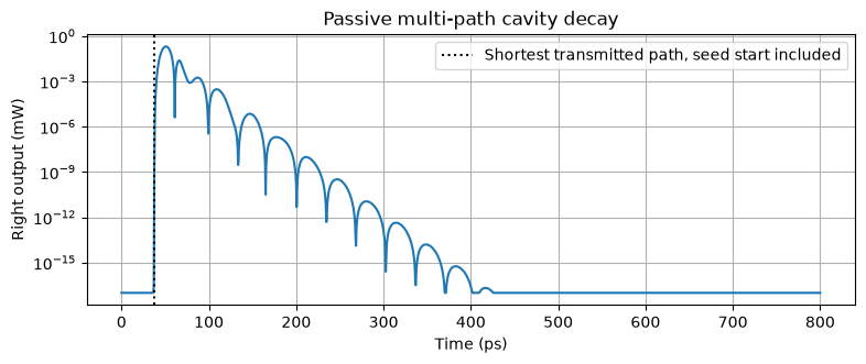
We compare complete startup power traces at identical saved times. Tests additionally check a pulse traversing a bidirectional waveguide in both directions with the expected delay and attenuation, and compare the full grating AC response with its analytic cascade. The passive assembled cavity below retains all grating internal reflections; it does not have a single universal echo time equal to twice the gain-region flight.
mesh = []
for cells in (2,4,8):
    device = circuit if cells==M else make_bench(p,s,cells)
    sol = transient(device,params)
    mesh.append(np.asarray(abs(device.port(sol.ys,"right"))**2))
space_errors = [np.linalg.norm(y-mesh[-1])/np.linalg.norm(mesh[-1]) for y in mesh[:-1]]
assert space_errors[1]<space_errors[0]
refined = []
for dt in (.6e-12,.3e-12,.15e-12):
    sol = transient(circuit,params,dt=dt)
    refined.append(np.asarray(abs(circuit.port(sol.ys,"right"))**2))
time_errors = [np.linalg.norm(y-refined[-1])/np.linalg.norm(refined[-1]) for y in refined[:-1]]
assert time_errors[1]<time_errors[0]
print("Space full-trace errors vs 8 gain cells (2,4):",space_errors)
print("Time full-trace errors vs 0.15 ps (0.6,0.3 ps):",time_errors)
fig, axes = plt.subplots(1,2,figsize=(10,3.2),constrained_layout=True)
for cells,y in zip((2,4,8),mesh):axes[0].plot(times*1e9,y*1e3,label=f"{cells} gain cells")
for dt,y in zip((.6,.3,.15),refined):axes[1].plot(times*1e9,y*1e3,label=f"dt={dt} ps")
for ax in axes:ax.set(xlabel="Time (ns)",ylabel="Right output (mW)");ax.legend()
plt.show()

passive_p = p._replace(transparency_m3=0.,injection_efficiency=0.,saturation=0.,alpha_h=0.,detuning_rad_s=0.)
passive = make_bench(passive_p,s,M)
passive_sol = transient(passive,{"PUMP.dc":0.,"SEED.power_w":1e-3},end=.8e-9,dt=.15e-12,save_times=jnp.linspace(0,.8e-9,1601))
passive_power = np.asarray(abs(passive.port(passive_sol.ys,"right"))**2)
minimum_flight = flight+s.phase_length_m*s.passive_group_index/LIGHT_SPEED+(s.samples-1)*(1/(2*s.left_fsr_hz)+1/(2*s.right_fsr_hz))
assert np.max(passive_power[np.asarray(passive_sol.ts)<10e-12+minimum_flight-3e-12])<1e-10
assert passive_power[-100:].max()<passive_power.max()*1e-5
fig, ax = plt.subplots()
ax.semilogy(np.asarray(passive_sol.ts)*1e12,np.maximum(passive_power,1e-20)*1e3)
ax.axvline((10e-12+minimum_flight)*1e12,ls=":",color="k",label="Shortest transmitted path, seed start included")
ax.set(xlabel="Time (ps)",ylabel="Right output (mW)",title="Passive multi-path cavity decay")
ax.legend()
plt.show()
Space full-trace errors vs 8 gain cells (2,4): [np.float64(0.028857542840604763), np.float64(0.00591004509190807)]
Time full-trace errors vs 0.15 ps (0.6,0.3 ps): [np.float64(0.014030669954912698), np.float64(0.004794438838681891)]
A limiting check against independent lumped rate equations¤
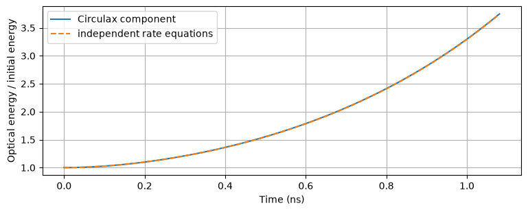
For weak single-pass loss, nearly uniform fields/carriers, and dynamics slow relative to flight time, the gain physics approaches lumped carrier/photon rate equations. The original native constant-facet component provides this restricted reference check below, using the same SOA material/depletion helpers as TravelingWaveGainCell. Its agreement does not replace convergence of the assembled dispersive cavity above: grating/ring energy storage generally prevents using the gain-region flight alone as the photon lifetime.
def make_circuit(settings, segments=8, *, matched_output=False, mirrors=None):
    netlist = {
        "instances": {
            "LASER": {"component": "laser", "settings": settings._asdict()},
            "PUMP": {"component": "pump"},
            "SEED": {"component": "seed", "settings": {"power_w": 0.0}},
            "GND": {"component": "ground"},
        },
        "connections": {
            "GND,p1": ("LASER,cathode", "PUMP,p1"),
            "PUMP,p2": "LASER,anode",
            "SEED,out": "LASER,seed",
        },
        "ports": {"left": "LASER,left", "right": "LASER,right"},
    }
    models = {
        "laser": TravelingWaveLaser if segments == 8 else traveling_wave_laser(segments),
        "pump": WaveformCurrentSource,
        "seed": CoherentSeed,
        "ground": lambda: 0,
    }
    if matched_output:
        netlist["instances"].update(
            {
                "WG": {"component": "waveguide", "settings": {"length_um": 500.0, "loss_dB_cm": 10.0, "wavelength_nm": 1540.0}},
                "LOAD": {"component": "load", "settings": {"R": 1.0}},
            }
        )
        netlist["connections"].update({"LASER,right": "WG,p1", "WG,p2": "LOAD,p1"})
        netlist["connections"]["GND,p1"] += ("LOAD,p2",)
        netlist["ports"]["received"] = "WG,p2"
        models.update({"waveguide": OpticalWaveguide, "load": Resistor})
    if mirrors is not None:
        netlist["instances"]["LASER"]["settings"].update(mirrors._asdict())
        netlist["instances"].update({"HP": {"component": "voltage"}, "HF": {"component": "voltage"}})
        netlist["connections"].update({"HP,p1": "LASER,heater_phase", "HF,p1": "LASER,heater_filter"})
        netlist["connections"]["GND,p1"] += ("HP,p2", "HF,p2", "LASER,heater_return")
        models.update({"laser": traveling_wave_laser(segments, tunable_mirrors=True), "voltage": VoltageSource})
    return compile_circuit(netlist, models, backend="klu", is_complex=True, g_leak=0.0, rtol=1e-10, atol=1e-12)
qsettings = p._replace(r_left=0.999 + 0j, r_right=0.999 + 0j, loss_m1=10, alpha_h=0)
qsettings = qsettings._replace(detuning_rad_s=float(resonant_detuning(qsettings)))
qc = make_circuit(qsettings, 4)
qgain, qnth, qith = threshold(qsettings)
qinitial = seeded_initial_state(qc, qc.dc(params={"PUMP.dc": 1.002 * qith}), qsettings, 4, seed_power_w=1e-5)
qtimes = jnp.linspace(0, 150 * flight, 151)
qsol = qc.transient(
    t0=0.0,
    t1=float(qtimes[-1]),
    dt0=flight / 8,
    y0=qinitial,
    saveat=qtimes,
    params={"PUMP.dc": 1.002 * qith},
    max_steps=1204,
    throw=True,
    transient_solver=TrapVectorizedTransientSolver(linear_solver=qc.solver, newton_rtol=1e-9, newton_atol=1e-12),
)
U = np.asarray(
    jnp.stack([abs(qc.port(qsol.ys, f"LASER,{direction}{j}")) ** 2 for direction in ("f", "b") for j in range(4)], axis=-1).sum(
        axis=-1
    )
    * flight
    / 4
)
velocity = LIGHT_SPEED / qsettings.group_index
volume = float(material_scales(qsettings)[0])
hv = PLANCK * LIGHT_SPEED / qsettings.wavelength_m


def rate_equations(t, y):
    N = y[0] * float(qnth)
    g = qsettings.confinement * qsettings.differential_gain_m2 * (N - qsettings.transparency_m3)
    dN = (
        qsettings.injection_efficiency * float(1.002 * qith) / (ELECTRON_CHARGE * volume)
        - N / qsettings.lifetime_s
        - velocity * g * y[1] * U[0] / (hv * volume)
    )
    return [dN / float(qnth), velocity * (g - float(qgain)) * y[1]]


reference = solve_ivp(rate_equations, (0, float(qtimes[-1])), (1, 1), t_eval=np.asarray(qtimes), rtol=1e-10, atol=1e-12)
np.testing.assert_allclose(U / U[0], reference.y[1], rtol=0.015)
print(f"Max relative energy difference: {np.max(abs(U / U[0] / reference.y[1] - 1)):.3%}")
fig, ax = plt.subplots()
ax.plot(qtimes * 1e9, U / U[0], label="Circulax component")
ax.plot(reference.t * 1e9, reference.y[1], "--", label="independent rate equations")
ax.set(xlabel="Time (ns)", ylabel="Optical energy / initial energy")
ax.legend()
plt.show()
Max relative energy difference: 0.143%
Wave ports, propagation and gain equations¤
Optical waves \(a,b\) have units √W. At each component port, \(a\) enters the device and \(b\) leaves it. Circulax stamps \(V=a+b\) and inward flow \(I=a-b\) at unit reference impedance. Connecting two ports enforces continuity of \(V\) and cancellation of \(I\), hence the outgoing wave of each becomes the incident wave of the other. Optical \(V,I\) are numerical wave coordinates, not electrical volts/amperes. At a matched unexcited output \(a=0\), so \(|V|^2\) is output power; inside a reflective circuit \(|V|^2\) is generally not directional power.
In a gain cell of length \(\Delta z=L/M\) (m), transit time \(\tau_g=\Delta z n_g/c\) (s), integrated modal gain \(h_j\) (dimensionless), and integrated passive power loss \(\ell=\alpha_i\Delta z\) (dimensionless), $\(b_R(t)=A_j(t)a_L(t-\tau_g),\qquad b_L(t)=A_j(t)a_R(t-\tau_g),\)$ $\(A_j=\exp\{[(1-i\alpha_H)h_j-\ell]/2+i(\Omega-\omega_F)\tau_g\},\)$ $\(\tau_c\dot h_j=h_{0j}(I_{Dj})-h_j-\frac{\tau_c}{E_{sat}}h_j\operatorname{exprel}(h_j-\ell)\,[|a_L(t-\tau_g)|^2+|a_R(t-\tau_g)|^2].\)$ Here \(\operatorname{exprel}(x)=(e^x-1)/x\), with limit 1 at zero. Both directions extract stimulated power from the same local carrier reservoir. This is the integral of the interference-averaged traveling-wave equations, using arrival-time gain uniform over a cell. Frozen retarded gain is a first-order spatial approximation; propagation at constant gain is exact apart from numerical history interpolation. Gain saturation is carrier depletion, with no separate ultrafast compression law.
| Symbol | Units | Physical role |
|---|---|---|
| \(L,\Delta z,w,d,A=wd,V=Lwd\) | m, m, m, m, m², m³ | Gain-region length, cell length, cross-section and active volume |
| \(c,n_g,v_g=c/n_g\) | m/s, 1, m/s | Vacuum light speed, group index and envelope group velocity |
| \(N_j,N_{tr}\) | m⁻³ | Carrier density and transparency |
| \(\Gamma,a\) | 1, m² | Confinement and differential material gain |
| \(g_j=h_j/\Delta z=\Gamma a(N_j-N_{tr})\) | m⁻¹ | Modal power gain |
| \(\alpha_i,\alpha_H\) | m⁻¹, 1 | Internal power loss and Henry phase/gain coupling |
| \(\tau_c,\eta,q\) | s, 1, C | Recombination lifetime, injection efficiency, elementary charge |
| \(I_{Dj},V_j\) | A, V | Cell diode conduction current and junction voltage |
| \(h_{0j}=\Gamma a[\eta I_{Dj}\tau_c/(q\Delta z A)-N_{tr}]\Delta z\) | 1 | Unsaturated integrated gain from conduction injection |
| \(h_P,\nu=c/\lambda_{ref},E_{sat}=h_P\nu A/(\Gamma a)\) | J·s, Hz, J | Planck constant, reference optical frequency and saturation energy |
| \(\Omega,\omega_F\) | rad/s | Fixed propagation calibration and envelope-frame offset |
The local diode follows the existing SOA: \(I_D=I_s s_A[\exp(V_j/(nV_T))-1]\), \(I_t=s_A(V_A-V_C-V_j)/R_s\), and \(C_js_A\dot V_j=I_t-I_D\), where \(s_A=\Delta z w/[(600\,\mu\mathrm m)(2\,\mu\mathrm m)]\). \(I_s\) (A), \(n\) (1), \(V_T\) (V), \(R_s\) (Ω), and \(C_j\) (F) default to \(10^{-12}\), 1.8, 0.02585, 5, and \(150\times10^{-15}\). \(V_A,V_C\) are contact voltages (V), and displacement current does not inject carriers. Parallel contacts distribute current in proportion to cell area.
Closure and omissions: carrier extraction uses \(|E_+|^2+|E_-|^2\). Optical reflection/interference is resolved in the passive network, but wavelength-scale standing-wave carrier gratings and their spatial hole burning in the gain region are averaged out. Gain bandwidth/dispersion, diffusion, transverse modes, nonlinear recombination, active-region self-heating and material-temperature dependence are omitted. Heating of passive sections is included. The deterministic seed gives no physical spontaneous-emission, linewidth or SMSR prediction.
Sampled gratings, phase section and thermal controls¤
A sampled reflector has \(K\) identical zero-length scattering patches separated by physical spacing \(D\) (m). Each patch is a reciprocal unitary two-port, $\(\binom{b_L}{b_R}=\begin{pmatrix}i\rho&t_p\\t_p&i\rho\end{pmatrix}\binom{a_L}{a_R},\qquad \rho=\tanh(\sigma/K),\quad t_p=\operatorname{sech}(\sigma/K).\)$ \(\sigma\) is dimensionless total grating strength, \(\rho\) is an amplitude magnitude, and \(t_p\) is an amplitude transmission. Unit-reflection conventions require the relative \(i\) phase. Each gap delays both directions by \(\tau_B=Dn_{gB}/c\) and multiplies the envelope by \(e^{i(\delta_B-\omega_F)\tau_B}\). Multiple reflections between patches are retained. For fixed temperature the gap response at physical angular-frequency offset \(\omega\) (rad/s) is \(z=e^{-i(\omega-\delta_B)\tau_B}\). Cascading a patch with a remaining reflector \((r,t)\) gives $\(r_{new}=i\rho+\frac{t_p^2 z^2r}{1-i\rho z^2r},\qquad t_{new}=\frac{t_p zt}{1-i\rho z^2r}.\)$ Here \(n_{gB}\) is the dimensionless passive grating group index (passive_group_index). The comb spacing is \(F=c/(2n_{gB}D)\) (Hz); peak power reflectance is \(\tanh^2\sigma\), whereas complex amplitude reflection is \(r(\omega)\). The physical reflector length is \((K-1)D\). The approximation neglects finite patch extent and its Bragg bandwidth. It retains delay and passivity without asserting an accurate fabricated grating spectrum. A sampled-grating laser experiment illustrates the two-comb Vernier principle.
Each heater obeys \(I_h=V_h/R_h\), \(P_h=V_h^2/R_h\), \(\tau_T\dot T=R_{th}P_h-T\). \(T\) is temperature rise (K), \(V_h\) voltage (V), \(I_h\) current (A), \(R_h\) resistance (Ω), \(P_h\) heat power (W), \(R_{th}\) thermal resistance (K/W), and \(\tau_T\) thermal time (s). The grating center is \(\lambda_B=\lambda_{ref}+k_\lambda T\) with \(k_\lambda\) in m/K, and \(\delta_B=2\pi c(1/\lambda_B-1/\lambda_{ref})\) in rad/s. Positive \(k_\lambda\) redshifts the comb. Temperature changes during one optical gap flight are neglected because thermal times are much longer.
The separate phase section has length \(L_p\) (m), delay \(\tau_p=L_p n_{gp}/c\) (s), and transmission $\(t_{\phi}(\omega)=e^{-\alpha_pL_p/2+i(\phi_0+k_\phi T_\phi)-i\omega\tau_p}.\)$ \(T_\phi\) is the phase-section temperature rise (K), and \(n_{gp}\) is its dimensionless group index. \(\alpha_p\) is power loss (m⁻¹), \(\phi_0\) fixed reference phase (rad), and \(k_\phi\) one-pass phase sensitivity (rad/K). In a shifted envelope frame the native delayed multiplier uses \(\phi_0+k_\phi T_\phi-\omega_F\tau_p\). Thermo-optic material dispersion, thermal cross-talk, tuning-induced absorption and optical absorption heating are omitted.
A optical interface uses \(r=i\rho_c A_c\), \(t=\sqrt{1-\rho_c^2}A_c\), where \(\rho_c\) is amplitude reflection magnitude and \(A_c=10^{-\mathcal L/20}\) for interface power loss \(\mathcal L\) (dB). Loss enters an implicit passive bath. The example has \(\rho_c=0\), so its analytic threshold helper applies. Introducing parasitic reflections is supported by the native component, but requires recomputing the whole network's mode condition.
Threshold, phase, solver limits and interpretation¤
For the reflection-free interfaces used here, four interface crossings per round trip give amplitude factor \(C=10^{-2\mathcal L/10}\). With complex grating reflections \(r_L,r_R\), $\(g_{th}=\alpha_i-\ln|C r_Lr_R|/L,\qquad I_{th}=qV[N_{tr}+g_{th}/(\Gamma a)]/(\eta\tau_c),\)$ $\(\mathcal A_{rt}=\frac{C r_Lr_R}{|C r_Lr_R|}\exp\{i[-\alpha_Hg_{th}L+2(\Omega-\omega)\tau_g^{gain}+2k_\phi T_\phi-2\omega\tau_p]\}=1.\)$ Here \(\tau_g^{gain}=Ln_g/c\). \(\mathcal A_{rt}\) is the unit-magnitude threshold round-trip field; its phase must also vanish modulo \(2\pi\). Reflection overlap alone does not solve that phase condition. Grating reflection phases include their propagation and energy storage. We enumerate phase crossings in a fixed ±1.1 THz validity window, retain thresholds up to 1.3 times the cold threshold current, and repeat with twice as many grid points. Near grating reflection zeros the flat, unbounded gain law generates very high thresholds and rapid Henry-phase windings; a finite current range is essential for qualifying the relevant roots. Sign-crossing searches can miss tangent roots; no global mode-count claim is made. Changing the window tests a different physical validity assumption for these indefinitely repeating ideal combs, rather than supplying a missing gain bandwidth.
The public solver already supports the required implicit delayed circuit feedback and different delays in different component instances. Each component currently supports one distinct delay duration, which is enough for a gain cell, one grating's repeated equal gaps, or one waveguide arm. General unequal-gap gratings should be assembled from additional cells, or the solver's delay representation must be extended. Complex non-holomorphic gain/heating uses real and imaginary blocks. Fixed time steps and linear accepted-history interpolation are used here; small integration steps are needed relative to field variation and the shortest significant flight. Newton tolerances are dimensionally scaled residual controls, not a spatial/time error estimate.
Every delayed leaf must use the same optical reference and frame: \(\nu_{opt}=c/\lambda_{ref}+\omega_F/(2\pi)+f_{env}\), where \(f_{env}\) is measured envelope phase slope/(2π), in Hz. hybrid_frame_parameters covers the default SG assembly. A replacement feedback network must shift its own delayed leaves consistently. Numerical tests check scattering conventions, passivity, two-way pulse delay/loss, carrier sharing, hierarchy, assembled startup/time/space convergence, and the seeded designed branch. Experimental calibration and physical SMSR remain separate work.