Push-pull traveling-wave MZM model¤
A Mach–Zehnder modulator (MZM) with differential-mode and common-mode electrodes is constructed and used to simulate a 56 Gbaud optical link with input and output grating couplers. The modulator is first driven with a binary signal; four-level pulse-amplitude modulation (PAM4) eye diagrams are then compared with and without transmitter timing jitter.
The modulator is built by cascading electro-optic unit cells along both arms. Each unit cell contains differential- and common-mode electrical half-lines, a modal-to-conductor adapter, and one four-port PN phase shifter per arm. Each phase shifter has an electrical anode and cathode and an optical input and output, with junction capacitance, a quadratic relationship between voltage and optical phase, optical loss, and propagation delay. The parameters are illustrative and would be replaced by extracted device data when a specific design is modeled.
The cells below define the components, assemble the circuit, and generate the drive waveforms. mode_transmission_line builds the electrode models, and DifferentialAdapter connects the modal voltages and currents to the physical junctions. A compact two-port line model is demonstrated in the reduced RLGC line example.
The binary drive uses a full 127-bit PRBS7 period and the PAM4 drive uses 128 data symbols, each after a 16-symbol preamble.
Eye diagrams show a binned density image with logarithmic colour scaling: each time column reports the fraction of folded traces in each amplitude bin. Both jitter cases use the same amplitude ranges.
# Copyright 2026 Circulax contributors

import copy
import time

import jax
import jax.numpy as jnp
import matplotlib.pyplot as plt
import numpy as np
from matplotlib.colors import LogNorm

from circulax import compile_circuit
from circulax.components import DifferentialAdapter, mode_transmission_line, phase_shifter_factory, pn_diode
from circulax.components.base_component import component
from circulax.components.electronic import (
    WAVE_DC,
    WAVE_PWL,
    WAVE_SIN,
    Resistor,
    WaveformVoltageSource,
)
from circulax.components.photonic import DirectionalCoupler, Grating, OpticalSource

jax.config.update("jax_enable_x64", True)
plt.rcParams.update({"figure.figsize": (10, 3.5), "axes.grid": True})
data_bits = 127
c0 = 299_792_458.0
length_m, n_sections = 2e-3, 6
dz = length_m / n_sections
baud = 56e9  # Symbol rate for the Nyquist metric and transient examples.
n_opt, wavelength_um, optical_loss_db_cm = 4.05, 1.55, 1.0
rj_product, cj_per_m = 4.7e-3, 320e-12  # ohm m, F/m
v_bias, phase_a1, phase_a2 = -1.0, 1.2, 0.15  # V, rad/(V mm), rad/(V² mm)
source_r = load_r = 30.0  # per conductor, ohms
laser_power, grating_loss_db = 1e-3, 3.0  # W, dB per grating
quadrature_phase = -np.pi / 2
print(f"{n_sections} sections: {dz * 1e6:.1f} um, Rj={rj_product / dz:.2f} ohm, Cj={cj_per_m * dz * 1e15:.1f} fF")
6 sections: 333.3 um, Rj=14.10 ohm, Cj=106.7 fF
1. Optical MZM¤
The optical circuit is constructed first. Two 50/50 couplers split the input light between two arms and recombine it at the output. The unused ports are terminated with matched 1 Ω optical-envelope loads. A separate phase shifter sets the relative phase between the arms:
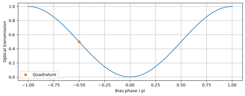
A constant phase is initially applied in each arm. For this wiring, the power transmission is \(P_\mathrm{out}/P_\mathrm{in}=[1-\cos(\theta)]/2\), where \(\theta\) is the relative arm phase. The sweep below verifies that \(\theta=-\pi/2\) gives quadrature bias: half transmission and maximum modulation slope.
@component(ports=("p1", "p2"), states=("a1", "a2"), holomorphic=True)
def PhaseBias(signals, phase=0.0):  # noqa: N802
    """Matched, reciprocal phase-only optical element; field impedance is 1 ohm."""
    transmission = jnp.exp(1j * phase)
    b1, b2 = transmission * signals.a2, transmission * signals.a1
    return {
        "p1": signals.a1 - b1,
        "p2": signals.a2 - b2,
        "a1": signals.p1 - signals.a1 - b1,
        "a2": signals.p2 - signals.a2 - b2,
    }, {}


def optical_netlist(arm_a, arm_b):
    return {
        "instances": {
            "GND": {"component": "ground"},
            "SPLIT": {"component": "coupler", "settings": {"coupling": 0.5}},
            "COMBINE": {"component": "coupler", "settings": {"coupling": 0.5}},
            "BIAS": {"component": "bias", "settings": {"phase": quadrature_phase}},
            "DUMP_IN": {"component": "R", "settings": {"R": 1.0}},
            "DUMP_OUT": {"component": "R", "settings": {"R": 1.0}},
        },
        "connections": {
            "SPLIT,p2": "DUMP_IN,p1",
            "DUMP_IN,p2": "GND,p1",
            "DUMP_OUT,p2": "GND,p1",
            "SPLIT,p3": arm_a[0],
            "SPLIT,p4": arm_b[0],
            arm_a[1]: "COMBINE,p1",
            arm_b[1]: "BIAS,p1",
            "BIAS,p2": "COMBINE,p2",
            "COMBINE,p4": "DUMP_OUT,p1",
        },
        "ports": {"optical_in": "SPLIT,p1", "optical_out": "COMBINE,p3"},
    }
optical_models = {"coupler": DirectionalCoupler, "bias": PhaseBias, "R": Resistor}
simple_net = optical_netlist(("ARM_A,p1", "ARM_A,p2"), ("ARM_B,p1", "ARM_B,p2"))
simple_net["instances"].update(ARM_A={"component": "bias"}, ARM_B={"component": "bias"})
simple_mzm = compile_circuit(simple_net, optical_models, is_complex=True)
static_net = {
    "instances": {
        "GND": {"component": "ground"},
        "MZM": {"component": "mzm"},
        "LASER": {"component": "laser", "settings": {"power": laser_power}},
        "LOAD": {"component": "R", "settings": {"R": 1.0}},
    },
    "connections": {"LASER,p1": "MZM,optical_in", "LASER,p2": "GND,p1", "MZM,optical_out": "LOAD,p1", "LOAD,p2": "GND,p1"},
    "ports": {"output": "LOAD,p1"},
}
static = compile_circuit(static_net, {"mzm": simple_mzm, "laser": OpticalSource, "R": Resistor}, is_complex=True)
phases = jnp.linspace(-np.pi, np.pi, 41)
static_solution = static.dc(params={"MZM~BIAS.phase": phases})
transmission = np.abs(np.asarray(static.port(static_solution, "output"))) ** 2 / laser_power
np.testing.assert_allclose(transmission, (1 - np.cos(phases)) / 2, atol=1e-7)
plt.plot(phases / np.pi, transmission)
plt.plot(-0.5, 0.5, "o", label="Quadrature")
plt.xlabel("Bias phase / pi")
plt.ylabel("Optical transmission")
plt.legend()
plt.show()
2. Modal transmission lines¤
The two coupled conductor signals of the uniform, symmetric electrode pair are decomposed into differential and common modes. Adapters convert between the modal and physical-conductor representations, following the mixed-mode treatment in Peter J. Pupalaikis, S-Parameters for Signal Integrity (Cambridge University Press, 2020), Chapter 7, especially Sections 7.3–7.4. The modal voltages and currents are defined as
With these definitions, two 30 Ω conductor terminations are equivalent to 60 Ω in differential mode and 15 Ω in common mode. Extracted per-conductor odd-mode and even-mode impedances are converted using \(Z_d=2Z_\mathrm{odd}\) and \(Z_c=Z_\mathrm{even}/2\).
mode_transmission_line accepts each of the following inputs as a function, a sampled array, or a scalar:
| Input | Unit |
|---|---|
attenuation_db_per_m | dB/m |
n_eff — RF phase index | dimensionless |
impedance — real or complex characteristic impedance | Ω |
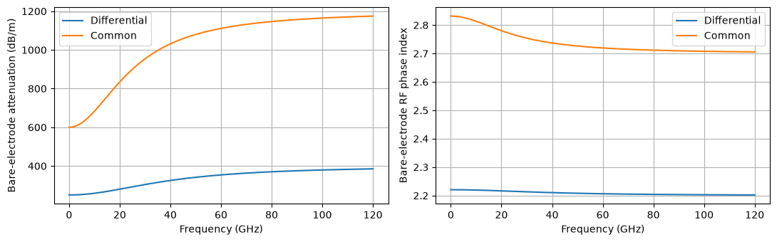
The factory fits these inputs and constructs a passive resistor–inductor–capacitor (RLC) line model. This example uses bare-electrode data, and the PN junction resistance and capacitance are added in the next step. When extracted mode data already include those junction elements, the additional electrical loading is omitted while the optical phase response is retained.
The illustrative common mode has higher loss, a larger phase index, and a different impedance than the differential mode. The parameters are chosen so that the loaded differential mode approximately matches the optical propagation velocity. For a specific device, both modes would be extracted from its electrode and return-path geometry.
frequencies = np.r_[0.0, np.geomspace(1e7, 120e9, 200)]


def attenuation_d(f_hz):
    """Illustrative differential-mode attenuation, in dB/m."""
    x = f_hz / 40e9
    return 250.0 + 150.0 * x**2 / (1 + x**2)


def neff_d(f_hz):
    return 2.2 + 0.0206 / (1 + (f_hz / 40e9) ** 2)


def attenuation_c(f_hz):
    x = f_hz / 25e9
    return 600.0 + 600.0 * x**2 / (1 + x**2)


def neff_c(f_hz):
    return 2.7 + 0.1318 / (1 + (f_hz / 25e9) ** 2)


# An extracted Z(f) array or callable can replace either constant impedance.
line_d = mode_transmission_line(frequencies, attenuation_db_per_m=attenuation_d, n_eff=neff_d, impedance=110.0)
line_c = mode_transmission_line(frequencies, attenuation_db_per_m=attenuation_c, n_eff=neff_c, impedance=45.0)
half_d, half_c = line_d(length=dz / 2), line_c(length=dz / 2)

fig, axes = plt.subplots(1, 2, figsize=(11, 3.5))
for label, attenuation, index, line in (
    ("Differential", attenuation_d, neff_d, line_d),
    ("Common", attenuation_c, neff_c, line_c),
):
    axes[0].plot(frequencies / 1e9, attenuation(frequencies), label=label)
    axes[1].plot(frequencies / 1e9, index(frequencies), label=label)
    print(f"{label} fit NRMSE: series {line.series.normalized_rmse:.3%}, shunt {line.shunt.normalized_rmse:.3%}")
axes[0].set(xlabel="Frequency (GHz)", ylabel="Bare-electrode attenuation (dB/m)")
axes[1].set(xlabel="Frequency (GHz)", ylabel="Bare-electrode RF phase index")
axes[0].legend()
axes[1].legend()
plt.tight_layout()
plt.show()
Differential fit NRMSE: series 0.026%, shunt 0.026%
Common fit NRMSE: series 0.023%, shunt 0.023%
3. Junction phase shifters¤
At each section midpoint, a DifferentialAdapter connects the two modal lines to the physical conductors. The adapter preserves power as it converts voltages and currents between the modal and conductor representations, allowing the junction currents to load both lines.
The schematic shows one electro-optic unit cell of length \(\Delta z\). D/C denote the modal ports; a (+) and b (−) denote the physical conductor ports. Each PN phase shifter has four ports: electrical anode and cathode, and optical o1 and o2. Its electrical current and charge load the electrode, while the junction voltage sets the optical phase and loss. Each optical section also includes propagation delay.
Cascade cells by connecting d_out to the next cell's d_in, c_out to c_in, and each arm's o2 to the next cell's o1. The cathodes remain grounded locally. With \(N\) cells, the total device length is \(L=N\Delta z\); the two adjacent electrical half-lines span \(\Delta z\) between section midpoints. The lower diagram shows these four connections between successive cells.
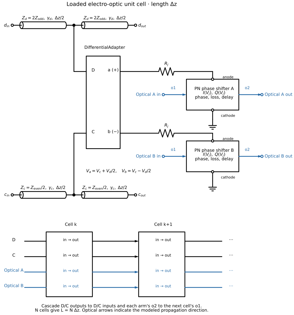
Each four-port PN phase shifter combines an electrical junction model at anode and cathode with an optical propagation model between o1 and o2. The junction voltage couples the two models; the series resistance \(R_j\) shown in the schematic is a separate component.
The junction is an electrical model that can be constructed and checked independently. pn_diode combines the diode equation, a depletion capacitance \(C_j(V)\), and a dark (reverse leakage) current, all per metre of junction length:
\(C_{j0}\) is chosen so that the capacitance at the operating bias matches the extracted value, and the I–V and C–V curves are plotted before the diode is used in the modulator. For measured data, junction_model(current=..., charge=charge_from_capacitance_table(v, c)) accepts arbitrary functions and tables instead.
The optics are functions of the junction voltage \(V_j=V_\mathrm{anode}-V_\mathrm{cathode}\):
| Input | Returns | Unit |
|---|---|---|
delta_neff | change in optical effective index; by convention it increases under reverse bias | dimensionless |
loss_dB_cm | optical propagation loss | dB/cm |
junction | the electrical model above, or None for a junction-free (Pockels) modulator | — |
Each input can be a function or a constant. Keyword arguments of the supplied functions, such as a1 and a2 below, and the diode parameters become settings of every phase-shifter instance, and can therefore be set in the netlist, swept, or fitted with JAX gradients. delta_neff_from_vpil integrates a small-signal VπL(V) table, and tabulated interpolates a Δn_eff(V) or loss(V) table, for example from a 2D carrier and mode simulation.
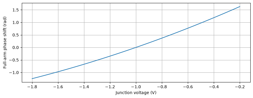
This example uses a quadratic phase response, written as an effective-index change,
and a constant optical loss. Here, \(\Delta z_\mathrm{mm}\) is the section length in millimetres, and \(a_1\) and \(a_2\) set the linear and quadratic phase response. The bias parameter sets the phase reference; the electrical DC solution determines the actual junction voltage.
Each section delays light by its optical transit time and applies the voltage-dependent phase at its midpoint, using the junction voltage from when the light passed it.
vbi, grading = 0.9, 0.5  # V, dimensionless
diode = pn_diode(
    cj0_F_per_m=cj_per_m * (1 - v_bias / vbi) ** grading,  # C_j(v_bias) = cj_per_m
    vbi=vbi,
    grading=grading,
    dark_current_A_per_m=1e-5,  # 10 nA/mm at the dark_bias_V reference
    dark_bias_V=-1.0,
)

v_diode = np.linspace(-2.0, 0.6, 261)
fig, axes = plt.subplots(1, 2, figsize=(11, 3.5))
axes[0].semilogy(v_diode, np.abs(diode.current(v_diode)) * length_m * 1e9)
axes[0].set(xlabel="Junction voltage (V)", ylabel="|Current| for one arm (nA)")
axes[1].plot(v_diode, diode.capacitance(v_diode) * 1e12)
axes[1].axvline(v_bias, color="k", linestyle="--", label="Bias")
axes[1].set(xlabel="Junction voltage (V)", ylabel="Capacitance (pF/m = fF/mm)")
axes[1].legend()
plt.tight_layout()
plt.show()
print(
    f"C_j({v_bias} V) = {float(diode.capacitance(v_bias)) * 1e12:.1f} pF/m; arm dark current {float(-diode.current(-1.0)) * length_m * 1e9:.1f} nA"
)
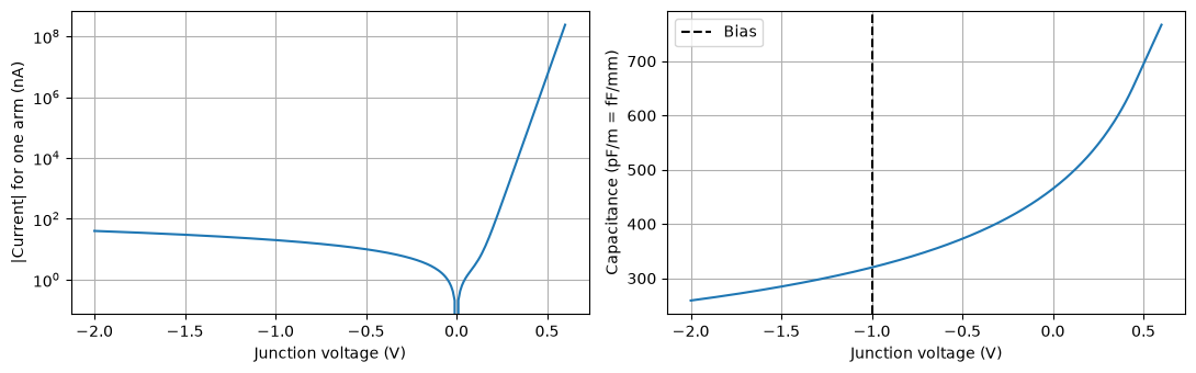
C_j(-1.0 V) = 320.0 pF/m; arm dark current 20.0 nA
def delta_neff(v, a1=phase_a1, a2=phase_a2, bias=v_bias):
    """Quadratic phase efficiency, a1 in rad/(V mm) and a2 in rad/(V² mm), as an index change."""
    phase_per_m = 1e3 * (a1 * (v - bias) + a2 * (v**2 - bias**2))
    return -phase_per_m * wavelength_um * 1e-6 / (2 * np.pi)


PNPhaseShifter = phase_shifter_factory(
    delta_neff=delta_neff,
    loss_dB_cm=optical_loss_db_cm,
    junction=diode,
    name="PNPhaseShifter",
)
phase_settings = {
    "length_um": dz * 1e6,
    "n_group": n_opt,
    "wavelength_nm": wavelength_um * 1e3,
    "a1": phase_a1,
    "a2": phase_a2,
    "bias": v_bias,
}
v_plot = np.linspace(-1.8, -0.2, 101)
plt.plot(v_plot, length_m * 1e3 * (phase_a1 * (v_plot - v_bias) + phase_a2 * (v_plot**2 - v_bias**2)))
plt.xlabel("Junction voltage (V)")
plt.ylabel("Full-arm phase shift (rad)")
plt.show()
def electrode_netlist(*, n_sections: int, dz: float, rj_product: float, phase_settings: dict | None = None) -> dict:
    """Repeat modal half-lines, an adapter and two Rj/junction branches.

    Without phase_settings each junction is the electrical diode alone.
    Supplying phase_settings uses PN phase shifters instead and connects
    the optical sections along each arm.
    """
    optical = phase_settings is not None
    net = {"instances": {"GND": {"component": "ground"}}, "connections": {}, "ports": {}}
    ins, con, ports = net["instances"], net["connections"], net["ports"]
    for k in range(n_sections):
        ins[f"X{k}"] = {"component": "adapter"}
        for mode, model in (("d", "d_line"), ("c", "c_line")):
            left, right = f"{mode}L{k}", f"{mode}R{k}"
            ins[left], ins[right] = {"component": model}, {"component": model}
            con[f"{left},p2"] = f"X{k},{mode}"
            con[f"{right},p1"] = f"X{k},{mode}"
            if k:
                con[f"{left},p1"] = f"{mode}R{k - 1},p2"
            else:
                ports[f"{mode}_in"] = f"{left},p1"
            ports[f"{mode}_out"] = f"{right},p2"
        for arm in ("a", "b"):
            resistor, junction = f"R{arm}{k}", f"PS{arm}{k}"
            ins[resistor] = {"component": "R", "settings": {"R": rj_product / dz}}
            ins[junction] = (
                {"component": "pn", "settings": phase_settings}
                if optical
                else {"component": "junction", "settings": {"length_um": dz * 1e6}}
            )
            con[f"{resistor},p1"] = f"X{k},{arm}"
            con[f"{resistor},p2"] = f"{junction},anode"
            con[f"{junction},cathode"] = "GND,p1"
            ports[f"junction_{arm}_{k}"] = f"{junction},anode"
    if optical:
        for arm in ("a", "b"):
            for k in range(n_sections - 1):
                con[f"PS{arm}{k},o2"] = f"PS{arm}{k + 1},o1"
    return net
electrode_settings = {"n_sections": n_sections, "dz": dz, "rj_product": rj_product}
models = {
    **optical_models,
    "adapter": DifferentialAdapter,
    "pn": PNPhaseShifter,
    "junction": diode.component("PNJunction"),
    "d_line": half_d,
    "c_line": half_c,
}
electrical_net = electrode_netlist(**electrode_settings)
electrical = compile_circuit(electrical_net, models, is_complex=False)
4. Bias and electrical checks¤
An electrical test circuit is constructed with the driver and terminations outside the MZM. VD drives the differential mode, while VC supplies the common-mode bias. The DC operating point is solved first, and the junction voltages along both arms are inspected. Electrode resistance and leakage can shift these voltages from the ideal source/load divider values.
A single-frequency electrical check uses the same cascaded unit cells with each four-port PN phase shifter replaced by its two-terminal junction, diode.component(). It verifies that a differential drive produces no common-mode junction voltage and vice versa. This checks modal wiring and junction loading. The full EO frequency response is computed after the optical link is assembled, using the quadrature-aware small_signal() interface.
def electrical_bench():
    return {
        "instances": {
            "GND": {"component": "ground"},
            "MZM": {"component": "mzm"},
            "VD": {"component": "drive", "settings": {"dc": 0.0}},
            "VC": {"component": "drive", "settings": {"dc": 2 * v_bias}},
            "RD": {"component": "R", "settings": {"R": 2 * source_r}},
            "RC": {"component": "R", "settings": {"R": source_r / 2}},
            "LD": {"component": "R", "settings": {"R": 2 * load_r}},
            "LC": {"component": "R", "settings": {"R": load_r / 2}},
        },
        "connections": {
            "VD,p1": "RD,p1",
            "RD,p2": "MZM,d_in",
            "MZM,d_out": "LD,p1",
            "VC,p1": "RC,p1",
            "RC,p2": "MZM,c_in",
            "MZM,c_out": "LC,p1",
            "VD,p2": "GND,p1",
            "VC,p2": "GND,p1",
            "LD,p2": "GND,p1",
            "LC,p2": "GND,p1",
        },
        "ports": {f"junction_{arm}_{k}": f"MZM,junction_{arm}_{k}" for arm in ("a", "b") for k in range(n_sections)},
    }
bench_models = {"R": Resistor, "drive": WaveformVoltageSource}
rf = compile_circuit(electrical_bench(), {**bench_models, "mzm": electrical}, is_complex=False)
rf_dc = rf.dc()
bias_a = np.array([float(rf.port(rf_dc, f"junction_a_{k}")) for k in range(n_sections)])
bias_b = np.array([float(rf.port(rf_dc, f"junction_b_{k}")) for k in range(n_sections)])
np.testing.assert_allclose(bias_a, bias_b, atol=1e-8)
print(f"Junction bias along either arm: {bias_a.round(3)} V")
# Check modal wiring without treating the last junction as the EO output.
for source in ("VD", "VC"):
    ac = rf.ac_response(freqs=jnp.asarray([28e9]), sources={source: 1.0}, y_dc=rf_dc)
    va = np.asarray(rf.port(ac["solution"], f"junction_a_{n_sections - 1}"))
    vb = np.asarray(rf.port(ac["solution"], f"junction_b_{n_sections - 1}"))
    rejected_voltage = (va + vb) / 2 if source == "VD" else va - vb
    assert np.max(abs(rejected_voltage)) < 1e-7
Junction bias along either arm: [-1.12 -1.061 -1.004 -0.947 -0.89 -0.834] V
Velocity matching¤
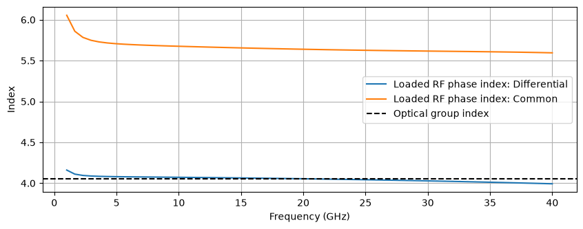
For push-pull operation, the loaded differential RF phase index is compared with the optical group index. At each modulation frequency \(f\), the light sees the RF wave's phase accumulate as \(\beta_\mathrm{RF}(f)z\), set by the RF phase index, while the modulation travels with the optical envelope at the optical group velocity. The walk-off phase is therefore \(2\pi f L[n_\mathrm{RF}(f)-n_{g,\mathrm{opt}}]/c\). The common mode has a different delay, which affects the response to common-mode ripple.
The helper below calculates the phase index from the propagation constant of the repeated RLC section, including the junction resistance, the diode capacitance at the bias voltage, and section discretization. In this example, the added capacitance slows the RF wave relative to the bare electrode. When extracted mode data already include junction loading, the extracted n_eff is compared directly with the optical group index.
def loaded_phase_index(line, frequencies, *, scale: float, dz: float, rj_product: float, cj_per_m: float) -> np.ndarray:
    """RF phase index from the Bloch propagation constant of a symmetric, junction-loaded RLC cell.

    scale converts the physical junction to differential (2) or common (0.5)
    mode: R_modal = scale * Rj and C_modal = Cj / scale.
    """
    f = np.asarray(frequencies)
    s_ac = 2j * np.pi * f
    d = dz / 2
    series = np.tile(np.eye(2, dtype=complex), (len(f), 1, 1))
    shunt = series.copy()
    series[:, 0, 1] = line.series.evaluate(f) * d / 2
    shunt[:, 1, 0] = line.shunt.evaluate(f) * d
    half = series @ shunt @ series
    junction = np.tile(np.eye(2, dtype=complex), (len(f), 1, 1))
    junction[:, 1, 0] = s_ac * (cj_per_m * dz / scale) / (1 + s_ac * rj_product * cj_per_m)
    cell = half @ junction @ half
    gamma_loaded = np.arccosh((cell[:, 0, 0] + cell[:, 1, 1]) / 2) / dz
    return 299_792_458.0 * gamma_loaded.imag / (2 * np.pi * f)
velocity_frequencies = jnp.linspace(1e9, 40e9, 61)
fig, ax = plt.subplots()
for label, line, scale in (("Differential", line_d, 2.0), ("Common", line_c, 0.5)):
    cj_bias = float(diode.capacitance(v_bias))
    phase_index = loaded_phase_index(line, velocity_frequencies, scale=scale, dz=dz, rj_product=rj_product, cj_per_m=cj_bias)
    ax.plot(np.asarray(velocity_frequencies) / 1e9, phase_index, label=f"Loaded RF phase index: {label}")
    design = np.argmin(abs(np.asarray(velocity_frequencies) - 20e9))
    walkoff_ps = length_m * (phase_index[design] - n_opt) / c0 * 1e12
    print(
        f"{label} near 20 GHz: loaded RF phase index {phase_index[design]:.3f}, optical group index {n_opt:.3f}; walk-off {walkoff_ps:.2f} ps"
    )
ax.axhline(n_opt, color="k", linestyle="--", label="Optical group index")
ax.set(xlabel="Frequency (GHz)", ylabel="Index")
ax.legend()
plt.show()
Differential near 20 GHz: loaded RF phase index 4.055, optical group index 4.050; walk-off 0.03 ps
Common near 20 GHz: loaded RF phase index 5.639, optical group index 4.050; walk-off 10.60 ps
5. Traveling-wave MZM assembly¤
The constant-phase arms are replaced with n_sections cascaded electro-optic unit cells, with \(N\) denoting the number of cells and \(\Delta z=L/N\) their length, as shown in the schematic above. Each cell contains the two modal half-lines on either side of a midpoint adapter and one four-port PN phase shifter per arm. Adjacent cells share the differential- and common-mode line connections, and each arm's optical o2 connects to the next cell's o1. The phase shifters' cathodes connect to ground, and their anodes connect to the local adapter through \(R_j\).
The splitter, combiner, and bias phase shifter are retained around the cascaded arms. The resulting subcircuit exposes the first and last optical ports of each arm through the splitter and combiner, the differential- and common-mode RF ports at both electrode ends, and the junction-voltage monitors.
mzm_net = electrode_netlist(**electrode_settings, phase_settings=phase_settings)
optical = optical_netlist(("PSa0,o1", f"PSa{n_sections - 1},o2"), ("PSb0,o1", f"PSb{n_sections - 1},o2"))
for key in ("instances", "connections", "ports"):
    mzm_net[key].update(optical[key])
mzm = compile_circuit(mzm_net, models, is_complex=True, rtol=1e-9, atol=1e-10)
print("MZM ports:", [p for p in mzm.ports if not p.startswith("junction")])
MZM ports: ['c_in', 'c_out', 'd_in', 'd_out', 'optical_in', 'optical_out']
6. Grating couplers¤
The MZM is placed between a continuous-wave (CW) laser and an optical load, with a grating coupler at each end:
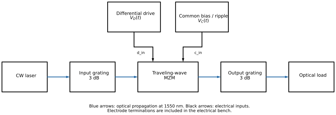
The compiled MZM is added to the link circuit's model dictionary. Each grating contributes 3 dB of loss at 1550 nm. Power is monitored both before and after the output grating to quantify its contribution to the link loss. These grating models do not include envelope dispersion.
link_net = electrical_bench()
link_net["instances"].update(
    {
        "LASER": {"component": "laser", "settings": {"power": laser_power}},
        "GRATING_IN": {
            "component": "grating",
            "settings": {"peak_loss_dB": grating_loss_db, "center_wavelength_nm": 1550.0, "wavelength_nm": 1550.0},
        },
        "GRATING_OUT": {
            "component": "grating",
            "settings": {"peak_loss_dB": grating_loss_db, "center_wavelength_nm": 1550.0, "wavelength_nm": 1550.0},
        },
        "OPTICAL_LOAD": {"component": "R", "settings": {"R": 1.0}},
    }
)
link_net["connections"].update(
    {
        "LASER,p1": "GRATING_IN,grating",
        "LASER,p2": "GND,p1",
        "GRATING_IN,waveguide": "MZM,optical_in",
        "MZM,optical_out": "GRATING_OUT,waveguide",
        "GRATING_OUT,grating": "OPTICAL_LOAD,p1",
        "OPTICAL_LOAD,p2": "GND,p1",
    }
)
link_net["ports"].update(output="OPTICAL_LOAD,p1", mzm_output="MZM,optical_out")
link_models = {**bench_models, "mzm": mzm, "laser": OpticalSource, "grating": Grating}
link = compile_circuit(link_net, link_models, is_complex=True, rtol=1e-9, atol=1e-10)
op = link.dc()
received_dc = float(abs(link.port(op, "output")) ** 2)
max_received = laser_power * 10 ** (-(2 * grating_loss_db + optical_loss_db_cm * length_m * 100) / 10)
np.testing.assert_allclose(received_dc, max_received / 2, rtol=1e-6)
print(f"Received power at quadrature: {received_dc * 1e3:.4f} mW")
Received power at quadrature: 0.1199 mW
Differential input to optical output: EO response and detected S31¤
The main frequency response is the modulation of the MZM optical output, including the contribution of every phase-shifter section and the propagation delay between sections. A voltage trace at the last junction cannot capture that distributed electro-optic interaction.
Number the differential electrode input port 1 and its terminated output port 2. First use the MZM optical output, before the output grating, as observation plane 3. link.small_signal(y_dc=op) linearizes the full electro-optic circuit at the DC bias. Driving only VD gives the complex optical-power modulation \(\delta P_3(f)\); the common-mode source retains its bias with zero AC excitation. Both optical field quadratures are included. The EO transfer per open-circuit source volt is
This is a dimensional EO transfer, rather than an electrical power-wave S-parameter. To define a dimensionless detected \(S_{31}\), place an ideal photodetector of responsivity \(\mathcal R\) at observation plane 3, delivering its photocurrent into a real receiving reference/load \(Z_3\). The detector is modeled here by postprocessing optical power; it adds no optical reflection, bandwidth limit, or electrical feedback. With the source resistance equal to the real differential reference \(Z_1=2R_s=60\,\Omega\) and no incident waves at the other electrical ports,
The RF normalization follows the standard power-wave definitions. The plots show normalized EO magnitude and the absolute magnitude and phase of detected \(S_{31}\). The detector values below are illustrative; absolute detected gain depends on optical input power, bias, responsivity, and the chosen reference impedances. A measured complex detector response can replace the constant \(\mathcal R\). The voltage-source phasor is a small-signal normalization and does not mean a 1 V nonlinear swing.
The output observation is also extracted after the output grating, for comparison with the subsequent HB and transient results. Both optical observations are power-normalized traveling fields here because the downstream optical loads are matched. The lower-level electrical checks above remain useful for validating modal wiring; they are not labeled EO response.
# Port 1: differential electrode input. Port 2: differential electrode output.
# Optical observation plane 3: MZM output, before the output grating.
eo_frequencies = jnp.r_[0.0, jnp.geomspace(0.1e9, 56e9, 81)]
eo_source_peak = 1.0  # V, open-circuit Thevenin source phasor; linearization only.
eo_model = link.small_signal(y_dc=op)
eo_response = eo_model(freqs=eo_frequencies, sources={"VD": eo_source_peak})
eo_power3 = eo_response.power("mzm_output", field_unit="sqrt(W)")
eo_received_power = eo_response.power("output", field_unit="sqrt(W)")
eo_h31 = eo_power3 / eo_source_peak  # Complex EO transfer in W/V of source drive.
eo_h31_received = eo_received_power / eo_source_peak
# Optical power modulation retains both field quadratures and RF phase.
eo_response_db = 20 * np.log10(np.abs(np.asarray(eo_h31 / eo_h31[0])))
eo_received_response_db = 20 * np.log10(np.abs(np.asarray(eo_h31_received / eo_h31_received[0])))

# An ideal, nonloading detector converts optical observation plane 3 into
# electrical port 3. These illustrative detector/reference values are explicit.
eo_responsivity = 0.8  # A/W; replace with the measured complex R_PD(f) if needed.
eo_z1, eo_z3 = 2 * source_r, 50.0  # ohms; real reference impedances.
eo_a1 = eo_source_peak / (2 * np.sqrt(eo_z1))
eo_v3 = eo_responsivity * eo_z3 * eo_power3  # PD current delivered into Z3.
eo_b3 = eo_v3 / np.sqrt(eo_z3)  # Matched receiving load: a3 = 0.
eo_s31 = eo_b3 / eo_a1
np.testing.assert_allclose(
    eo_s31, 2 * eo_responsivity * np.sqrt(eo_z1 * eo_z3) * eo_h31, rtol=1e-12
)

# Check the zero-frequency EO transfer against the full optical DC slope.
eo_dc_step = 1e-4
check_dc = link.dc(params={"VD.dc": jnp.array([-eo_dc_step, eo_dc_step])})
check_power = np.abs(np.asarray(link.port(check_dc, "mzm_output"))) ** 2
check_slope = (check_power[1] - check_power[0]) / (2 * eo_dc_step)
np.testing.assert_allclose(eo_h31[0], check_slope, rtol=1e-4, atol=1e-10)
assert np.all(np.isfinite(np.asarray(eo_s31)))

fig, axes = plt.subplots(1, 3, figsize=(14, 4))
frequency_ghz = np.asarray(eo_frequencies[1:]) / 1e9
for ax, values, ylabel in zip(
    axes,
    (
        eo_response_db[1:],
        20 * np.log10(np.abs(np.asarray(eo_s31[1:]))),
        np.rad2deg(np.unwrap(np.angle(np.asarray(eo_s31))))[1:],
    ),
    ("Normalized EO response (dB)", "Detected S31, ideal PD (dB)", "Detected S31 phase (degrees)"),
):
    ax.semilogx(frequency_ghz, values)
    ax.set(xlabel="Modulation frequency (GHz)", ylabel=ylabel)
    nyquist_axis = ax.secondary_xaxis("top", functions=(lambda f: 2 * f, lambda rate: rate / 2))
    nyquist_axis.set_xlabel("Symbol rate at Nyquist (Gbaud)")
fig.suptitle("Differential input → full distributed MZM optical output", y=1.08)
fig.tight_layout()
plt.show()
print(f"DC EO transfer: {complex(eo_h31[0]):.4g} W/V of source drive")
print(f"DC detected S31: {20 * np.log10(abs(complex(eo_s31[0]))):.2f} dB (0.8 A/W, Z3 = 50 ohm)")
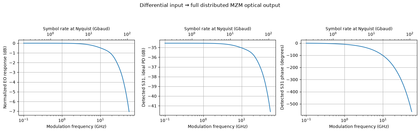
DC EO transfer: 0.0002135+0j W/V of source drive
DC detected S31: -34.56 dB (0.8 A/W, Z3 = 50 ohm)
7. Drive swing and 56 Gbaud transient¤
The drive amplitude is chosen to target a 4 dB extinction ratio (ER), defined as \(10\log_{10}(P_\mathrm{high}/P_\mathrm{low})\) between the settled outer optical power levels. The differential DC source is swept symmetrically about zero, with the optical circuit biased near quadrature, and the resulting transfer curve determines the source swing. This calibration includes electrode loading and the nonlinear phase response.
The common-mode source is held at its DC bias during calibration. differential_vpp is the full peak-to-peak differential source voltage; each conductor's source swing is half that value. Electrode loading reduces the swing that reaches the junctions.
target_er_db = 4.0
swing_vpp = jnp.linspace(0.0, 2.0, 101)
outer_dc = link.dc(params={"VD.dc": jnp.concatenate((-swing_vpp / 2, swing_vpp / 2))})
outer_power = np.abs(np.asarray(link.port(outer_dc, "output"))) ** 2
low, high = np.sort(outer_power.reshape(2, -1), axis=0)
er_sweep_db = 10 * np.log10(high / low)
assert np.all(np.diff(er_sweep_db) > 0)
assert er_sweep_db[-1] > target_er_db

differential_vpp = float(np.interp(target_er_db, er_sweep_db, np.asarray(swing_vpp)))
outer_dc = link.dc(params={"VD.dc": jnp.asarray([-differential_vpp / 2, differential_vpp / 2])})
outer_power = np.sort(np.abs(np.asarray(link.port(outer_dc, "output"))) ** 2)
calibrated_er_db = 10 * np.log10(outer_power[1] / outer_power[0])
np.testing.assert_allclose(calibrated_er_db, target_er_db, atol=0.01)
print(f"Differential source: {differential_vpp:.3f} Vpp; per conductor: {differential_vpp / 2:.3f} Vpp")
print(f"Settled outer powers: {outer_power * 1e3} mW; ER: {calibrated_er_db:.3f} dB")
Differential source: 0.998 Vpp; per conductor: 0.499 Vpp
Settled outer powers: [0.06830631 0.17157698] mW; ER: 4.000 dB
OMA and ER at Nyquist¤
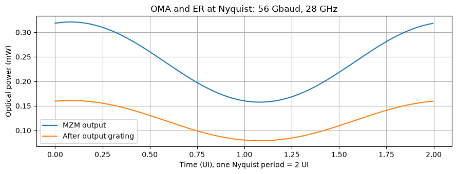
For a chosen symbol rate \(R_s\), evaluate the large-signal metric at one frequency, \(f_N=R_s/2\). The default baud=56e9 therefore gives 28 GHz. Harmonic balance solves the full electro-optic link for a sinusoidal differential source at the calibrated peak-to-peak swing, with the common-mode source held at its DC bias.
Report the optical modulation amplitude and extinction ratio at both the MZM output and after the output grating:
These are the sinusoidal OMA and ER at Nyquist, with a stated source swing and observation plane. They measure the finite-swing response at the target rate; the preceding small-signal EO sweep supplies the bandwidth curve. The flat output grating reduces OMA while preserving ER. The following PRBS/PAM4 examples measure data-waveform behavior separately.
Only one HB solve is needed. Reconstructing its complex optical envelope on a dense phase grid improves the measurement of power extrema without adding harmonics. Two harmonics are used here; increase nyquist_harmonics and rerun this cell to check convergence for a different drive swing or bias. The retained harmonics must stay inside the electrode model's fitted band. Change baud in the setup cell to evaluate another rate; it also sets the subsequent transient symbol rate.
The dense HB solver performance bottleneck is tracked separately in issue #105.
# Evaluate the large-signal metric at one Nyquist frequency, rather than sweeping HB.
nyquist_frequency = baud / 2
nyquist_harmonics = 2
assert nyquist_harmonics * nyquist_frequency <= np.max(frequencies), "Extend the electrode fit band or reduce the harmonic count."


def nyquist_fields(frequency):
    y_period, _ = link.hb(
        freq=frequency,
        harmonics=nyquist_harmonics,
        y0=op,
        params={
            "VD.kind": WAVE_SIN,
            "VD.offset": 0.0,
            "VD.amplitude": differential_vpp / 2,
            "VD.freq": frequency,
            "VC.kind": WAVE_DC,
        },
        max_steps=80,
    )
    return jnp.stack((link.port(y_period, "mzm_output"), link.port(y_period, "output")), axis=-1)


# One HB solve gives both optical observation planes.
nyquist_field_samples = jax.jit(nyquist_fields)(jnp.asarray(nyquist_frequency))
nyquist_phase = jnp.linspace(0.0, 2 * jnp.pi, 512, endpoint=False)
nyquist_samples = nyquist_field_samples.shape[0]
nyquist_orders = jnp.fft.fftfreq(nyquist_samples) * nyquist_samples
nyquist_coefficients = jnp.fft.fft(nyquist_field_samples, axis=0) / nyquist_samples
nyquist_fields_dense = jnp.exp(1j * nyquist_phase[:, None] * nyquist_orders) @ nyquist_coefficients
nyquist_power = np.asarray(jnp.abs(nyquist_fields_dense) ** 2)
assert np.all(np.isfinite(nyquist_power)) and np.all(nyquist_power > 0)
nyquist_low, nyquist_high = nyquist_power.min(axis=0), nyquist_power.max(axis=0)
nyquist_oma = nyquist_high - nyquist_low
nyquist_er_db = 10 * np.log10(nyquist_high / nyquist_low)

print(f"Nyquist metric: {baud / 1e9:g} Gbaud, f_N = {nyquist_frequency / 1e9:g} GHz")
print(f"Sinusoidal differential source: {differential_vpp:.3f} Vpp; HB harmonics: {nyquist_harmonics}")
print(f"{'Observation plane':<29} {'OMA (mW)':>12} {'ER (dB)':>12}")
for plane, oma, er in zip(("MZM output", "After output grating"), nyquist_oma, nyquist_er_db):
    print(f"{plane:<29} {oma * 1e3:12.5f} {er:12.3f}")

fig, ax = plt.subplots(figsize=(9, 3.5))
time_ui = np.asarray(nyquist_phase) / np.pi  # One Nyquist period spans two symbols.
ax.plot(time_ui, nyquist_power[:, 0] * 1e3, label="MZM output")
ax.plot(time_ui, nyquist_power[:, 1] * 1e3, label="After output grating")
ax.set(
    xlabel="Time (UI), one Nyquist period = 2 UI",
    ylabel="Optical power (mW)",
    title=f"OMA and ER at Nyquist: {baud / 1e9:g} Gbaud, {nyquist_frequency / 1e9:g} GHz",
)
ax.legend()
fig.tight_layout()
plt.show()
Nyquist metric: 56 Gbaud, f_N = 28 GHz
Sinusoidal differential source: 0.998 Vpp; HB harmonics: 2
Observation plane                 OMA (mW)      ER (dB)
MZM output                         0.16347        3.090
After output grating               0.08193        3.090
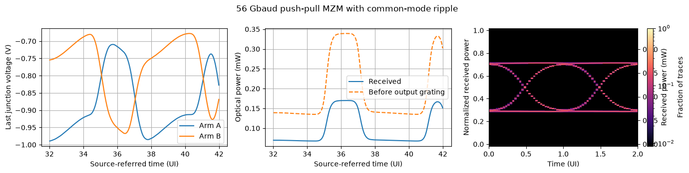
A seventh-order pseudorandom binary sequence (PRBS7) is generated, preceded by a constant 16-symbol preamble. One unit interval (UI) is one symbol period: approximately 17.86 ps at 56 Gbaud. Each voltage transition takes 0.2 UI. Setting common_ripple_vpp=0 disables the common-mode source ripple.
The transient starts from the operating point corresponding to the source levels at time zero. During the simulation, delayed signal values account for optical propagation and the local voltage-dependent phase response. Optical power is calculated as the squared field magnitude. Bandwidth limitations and common-mode ripple can make the dynamic extinction ratio differ from the DC calibration target.
def prbs_drive(baud, *, preamble_bits=16, vpp=4.0):
    """Return a PRBS7 pattern and 0.2-UI-edge differential PWL drive."""
    ui = 1 / baud
    state, pattern = 0x7F, []
    for _ in range(127):
        pattern.append(state & 1)
        state = (state >> 1) | (((state ^ (state >> 1)) & 1) << 6)
    if state != 0x7F or sum(pattern) != 64:
        msg = "Invalid PRBS7 period or balance"
        raise ValueError(msg)
    bits = np.r_[np.full(preamble_bits, pattern[0]), pattern[:data_bits]]
    levels = vpp * (bits - 0.5)
    times, values = [0.0], [float(levels[0])]
    for k in range(1, len(bits)):
        if levels[k] != levels[k - 1]:
            times.extend([k * ui, (k + 0.2) * ui])
            values.extend([float(levels[k - 1]), float(levels[k])])
    times.append(len(bits) * ui)
    values.append(float(levels[-1]))
    return bits, np.asarray(times), np.asarray(values)
samples_per_ui = 32
ui = 1 / baud
sample_dt, integration_dt = ui / samples_per_ui, ui / (2 * samples_per_ui)
preamble_bits, common_ripple_vpp = 16, 0.2
bits, pwl_t, pwl_v = prbs_drive(baud, preamble_bits=preamble_bits, vpp=differential_vpp)
print(f"NRZ record: {preamble_bits} preamble + {data_bits} data UI")
t_stop = len(bits) * ui
transient_net = copy.deepcopy(link_net)
transient_net["instances"]["VD"]["settings"] = {"kind": WAVE_PWL, "pwl_t": jnp.asarray(pwl_t), "pwl_v": jnp.asarray(pwl_v)}
transient_net["instances"]["VC"]["settings"] = {
    "kind": WAVE_SIN if common_ripple_vpp else WAVE_DC,
    "dc": 2 * v_bias,
    "offset": 2 * v_bias,
    "amplitude": common_ripple_vpp / 2,
    "freq": 10e9,
    "delay": preamble_bits * ui,
}
transient_link = compile_circuit(transient_net, link_models, is_complex=True, rtol=1e-9, atol=1e-10)
NRZ record: 16 preamble + 127 data UI
sample_times = jnp.arange(len(bits) * samples_per_ui + 1) * sample_dt
started = time.perf_counter()
solution = transient_link.transient(
    t0=0.0,
    t1=t_stop,
    dt0=integration_dt,
    saveat=sample_times,
    max_steps=int(np.ceil(t_stop / integration_dt)) + 20,
    throw=True,
)
solution.ys.block_until_ready()
power = np.abs(np.asarray(transient_link.port(solution.ys, "output"))) ** 2
mzm_power = np.abs(np.asarray(transient_link.port(solution.ys, "mzm_output"))) ** 2
np.testing.assert_allclose(power, mzm_power * 10 ** (-grating_loss_db / 10), rtol=1e-6, atol=1e-12)
assert np.all(np.isfinite(power))
assert power.max() <= max_received * 1.001
print(f"Transient: {time.perf_counter() - started:.1f} s; {solution.stats['num_steps']} steps")
Transient: 20.2 s; 9152 steps
8. Eye diagram¤
The junction voltages in both arms are plotted to confirm push-pull operation, and the received waveform is folded into two-UI windows to form an eye diagram. The preamble and the first eight data bits are excluded. Each window starts half a UI into a symbol, so that the display shows one complete eye in the center and half an eye on either side.
The known optical flight time is subtracted when the received waveform is aligned to the source clock. RF walk-off—the timing mismatch between electrical and optical propagation—and waveform distortion therefore remain visible.
The eye plot has axes for both normalized power and received power in milliwatts, including grating and waveguide losses. The power readout is ideal; receiver noise and equalization are not included.
def fold_eye(times, power, *, baud, samples_per_ui, preamble_bits, flight_time, center_ui=0.5):
    """Fold two UI with one central eye and half an eye at each edge.

    ``center_ui`` is the position within a symbol (0 to 1, after subtracting ``flight_time``) that is
    placed at the middle of the plot, so the crossings fall at 0.5 and 1.5 UI."""
    ui = 1 / baud
    n_bits = (len(times) - 1) // samples_per_ui
    eye_ui = np.arange(2 * samples_per_ui + 1) / samples_per_ui
    fold_bits = np.arange(preamble_bits + 8, n_bits - 5)
    query = flight_time + (fold_bits[:, None] + center_ui + eye_ui[None, :]) * ui
    if query.max() >= float(times[-1]):
        msg = "Eye windows extend beyond the simulated record"
        raise ValueError(msg)
    traces = np.interp(query.ravel(), times, power).reshape(query.shape)
    return eye_ui, traces

def plot_eye_density(ax, eye_ui, traces, *, ylim):
    """Bin folded samples into one image; colour is the fraction of traces per bin."""
    # The final point duplicates the start of the next two-UI window.
    values = np.asarray(traces)[:, :-1]
    counts, _, _ = np.histogram2d(
        np.broadcast_to(eye_ui[:-1], values.shape).ravel(),
        values.ravel(),
        bins=(eye_ui, np.linspace(*ylim, 161)),
    )
    density = counts.T / len(traces)
    ax.set_facecolor("black")
    ax.grid(False)
    return ax.imshow(
        np.ma.masked_equal(density, 0),
        origin="lower",
        extent=(eye_ui[0], eye_ui[-1], *ylim),
        aspect="auto",
        interpolation="nearest",
        cmap="magma",
        norm=LogNorm(vmin=1 / max(2, len(traces)), vmax=1),
    )
optical_flight = length_m * n_opt / c0
clock = (np.asarray(sample_times) - optical_flight) / ui
window = (clock >= preamble_bits + 16) & (clock <= preamble_bits + 26)
fig, axes = plt.subplots(1, 3, figsize=(14, 3.5))
for arm in ("a", "b"):
    voltage = np.asarray(transient_link.port(solution.ys, f"junction_{arm}_{n_sections - 1}")).real
    axes[0].plot(clock[window], voltage[window], label=f"Arm {arm.upper()}")
axes[0].set(xlabel="Source-referred time (UI)", ylabel="Last junction voltage (V)")
axes[0].legend()
axes[1].plot(clock[window], power[window] * 1e3, label="Received")
axes[1].plot(clock[window], mzm_power[window] * 1e3, "--", label="Before output grating")
axes[1].set(xlabel="Source-referred time (UI)", ylabel="Optical power (mW)")
axes[1].legend()
eye_ui, eye = fold_eye(
    np.asarray(sample_times),
    power,
    baud=baud,
    samples_per_ui=samples_per_ui,
    preamble_bits=preamble_bits,
    flight_time=optical_flight,
    center_ui=0.7,  # optical eye opens ~0.2 UI after the source edge; matches the 0.75-UI sampling point
)
image = plot_eye_density(axes[2], eye_ui, eye / max_received, ylim=(-0.02, 1.02))
fig.colorbar(image, ax=axes[2], label="Fraction of traces")
axes[2].set(xlabel="Time (UI)", ylabel="Normalized received power", xlim=(0, 2), ylim=(-0.02, 1.02))
axes[2].secondary_yaxis("right", functions=(lambda x: x * max_received * 1e3, lambda x: x / (max_received * 1e3))).set_ylabel(
    "Received power (mW)"
)
fig.suptitle("56 Gbaud push-pull MZM with common-mode ripple")
plt.tight_layout()
plt.show()
9. PAM4 drive with timing jitter¤
The same 56 Gbaud circuit and source swing, calibrated for 4 dB outer-level ER, are used. PAM4 has four equally spaced differential source voltages, differential_vpp * [-1/2, -1/6, 1/6, 1/2], and carries two bits per symbol: 112 Gb/s before coding. The nonlinear phase response remains active, so equally spaced source voltages need not produce equally spaced received optical powers. No predistortion is applied.
The same seeded sequence of 128 data symbols is compared with and without transmitter timing jitter:
random_jitter_ui: RMS Gaussian timing displacement in UI, clipped at three standard deviations.periodic_jitter_ui: peak sinusoidal timing displacement in UI, at frequencyperiodic_jitter_hz.
At 56 Gbaud, the defaults correspond to 0.45 ps RMS random jitter before clipping and 1.07 ps peak periodic jitter. The helper shifts each complete 0.2-UI transition ramp, preserving its duration and voltage levels. Jitter is applied to the electrical source before the circuit is simulated, so its effects propagate through the electrodes and phase shifters. Both cases retain the constant preamble and common-mode ripple.
Increasing n_symbols gives denser eye diagrams. This short record illustrates waveform distortion; it is too short to estimate a bit error rate (BER) or rare jitter events.
def pam4_drive(
    baud,
    *,
    n_symbols=128,
    preamble_symbols=16,
    vpp=4.0,
    random_jitter_ui=0.025,
    periodic_jitter_ui=0.06,
    periodic_jitter_hz=2e9,
    seed=7,
):
    """Return seeded PAM4 symbols and a PWL drive with jittered transition times.

    Random jitter is Gaussian with the specified RMS in UI, clipped at ±3 RMS.
    Periodic jitter is a sinusoidal time displacement with peak amplitude in UI.
    Both shift complete 0.2-UI ramps, preserving ramp duration and voltage levels.
    """
    rng = np.random.default_rng(seed)
    data = rng.integers(0, 4, n_symbols)
    symbols = np.r_[np.full(preamble_symbols, data[0]), data]
    levels = vpp * (symbols / 3 - 0.5)
    ui = 1 / baud
    edges = np.arange(1, len(symbols)) * ui
    random = np.clip(rng.normal(size=len(edges)), -3, 3) * random_jitter_ui
    periodic = periodic_jitter_ui * np.sin(2 * np.pi * periodic_jitter_hz * edges)
    shifts = ui * (random + periodic)
    shifts[edges < preamble_symbols * ui] = 0.0
    times, values = [0.0], [float(levels[0])]
    for k, start in enumerate(edges + shifts, start=1):
        if levels[k] != levels[k - 1]:
            times.extend([start, start + 0.2 * ui])
            values.extend([float(levels[k - 1]), float(levels[k])])
    times.append(len(symbols) * ui)
    values.append(float(levels[-1]))
    if np.any(np.diff(times) <= 0):
        msg = "Jitter is too large: PWL edges overlap or leave the simulation interval"
        raise ValueError(msg)
    return symbols, np.asarray(times), np.asarray(values)
n_symbols = 128
random_jitter_ui, periodic_jitter_ui, periodic_jitter_hz = 0.025, 0.06, 2e9
pam4_results = {}
for label, jitter_scale in (("No timing jitter", 0.0), ("With timing jitter", 1.0)):
    symbols, drive_t, drive_v = pam4_drive(
        baud,
        n_symbols=n_symbols,
        preamble_symbols=preamble_bits,
        vpp=differential_vpp,
        random_jitter_ui=jitter_scale * random_jitter_ui,
        periodic_jitter_ui=jitter_scale * periodic_jitter_ui,
        periodic_jitter_hz=periodic_jitter_hz,
        seed=7,
    )
    pam4_net = copy.deepcopy(transient_net)
    pam4_net["instances"]["VD"]["settings"].update(pwl_t=jnp.asarray(drive_t), pwl_v=jnp.asarray(drive_v))
    pam4_link = compile_circuit(pam4_net, link_models, is_complex=True, rtol=1e-9, atol=1e-10)
    pam4_times = jnp.arange(len(symbols) * samples_per_ui + 1) * sample_dt
    started = time.perf_counter()
    pam4_solution = pam4_link.transient(
        t0=0.0,
        t1=len(symbols) * ui,
        dt0=integration_dt,
        saveat=pam4_times,
        max_steps=2 * len(symbols) * samples_per_ui + 20,
        throw=True,
    )
    pam4_solution.ys.block_until_ready()
    received = np.abs(np.asarray(pam4_link.port(pam4_solution.ys, "output"))) ** 2
    assert np.all(np.isfinite(received))
    assert received.max() <= max_received * 1.001
    source = np.interp(np.asarray(pam4_times), drive_t, drive_v)
    pam4_results[label] = source, received
    settled_symbols = np.arange(preamble_bits + 8, len(symbols) - 5)
    sample_t = optical_flight + (settled_symbols + 0.75) * ui
    sampled_power = np.interp(sample_t, np.asarray(pam4_times), received)
    outer_levels = [np.median(sampled_power[symbols[settled_symbols] == level]) for level in (0, 3)]
    dynamic_er_db = abs(10 * np.log10(outer_levels[1] / outer_levels[0]))
    print(f"{label}: sampled outer-level ER {dynamic_er_db:.2f} dB")
    print(f"{label}: {time.perf_counter() - started:.1f} s; {pam4_solution.stats['num_steps']} steps")
No timing jitter: sampled outer-level ER 3.76 dB
No timing jitter: 17.8 s; 9216 steps


With timing jitter: sampled outer-level ER 3.77 dB
With timing jitter: 16.9 s; 9216 steps
fig, axes = plt.subplots(2, 2, figsize=(11, 6), sharex=True)
for row, (label, (source, received)) in enumerate(pam4_results.items()):
    for col, (signal, delay) in enumerate(((source, 0.0), (received * 1e3, optical_flight))):
        eye_ui, traces = fold_eye(
            np.asarray(pam4_times),
            signal,
            baud=baud,
            samples_per_ui=samples_per_ui,
            preamble_bits=preamble_bits,
            flight_time=delay,
            center_ui=0.7 if delay else 0.6,  # optical eye lags the 0.2-UI source ramp
        )
        limits = (
            (-0.55 * differential_vpp, 0.55 * differential_vpp)
            if col == 0
            else (-0.02 * max_received * 1e3, 1.02 * max_received * 1e3)
        )
        image = plot_eye_density(axes[row, col], eye_ui, traces, ylim=limits)
        fig.colorbar(image, ax=axes[row, col], label="Fraction of traces")
        axes[row, col].set(title=label, xlim=(0, 2))
    axes[row, 0].set_ylabel("Differential source (V)")
    axes[row, 1].set(ylabel="Received power (mW)", ylim=(-0.02 * max_received * 1e3, 1.02 * max_received * 1e3))
for ax in axes[-1]:
    ax.set_xlabel("Time (UI)")
fig.suptitle("56 Gbaud PAM4: electrical source and received optical eyes")
plt.tight_layout()
plt.show()
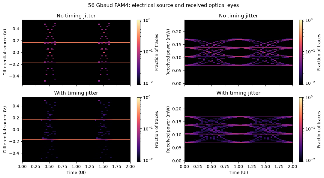
Both cases are folded against the same ideal symbol clock. The source eyes are centered 0.6 UI into each symbol (midway between the 0.2-UI ramps), and the optical eyes 0.7 UI in, where the received waveform settles. Each two-UI plot shows a complete eye in the center and half an eye on either side. Only the optical flight time is subtracted from the received waveform, so that transmitter jitter and RF walk-off remain visible.
The left column shows the electrical source eyes; the right column shows the received optical eyes. PAM4 produces three eye openings, one between each adjacent pair of levels. The opening heights indicate the level spacing, and the difference between the rows shows how timing jitter broadens the transitions. The printed dynamic ER uses median outer-level powers sampled 0.75 UI into each symbol after the initial settling interval. Receiver noise and clock recovery are not included.
The model can be explored by varying electrode attenuation, RF phase index, junction resistance and capacitance, common-mode ripple, or load resistance, and observing the effect on bandwidth, velocity matching, and the eye openings. Numerical convergence is checked by increasing n_sections and reducing integration_dt.
A line model without internal junction taps is demonstrated in the reduced RLGC line example, and a junction-free thin-film lithium niobate modulator in the TFLN traveling-wave MZM example.