Surface Models
Let's build some analytical surface models using MEOW and SAX
import json
from hashlib import md5
from pathlib import Path

import jax.numpy as jnp
import matplotlib.pyplot as plt
import meow as mw
import numpy as np
import pandas as pd
import xarray as xr
from tqdm.notebook import tqdm

import sax
Silicon Refractive index
Let's create a rudimentary silicon refractive index model:
def silicon_index(wl, T):
    """A rudimentary silicon refractive index model with temperature dependence"""
    a, b = 0.2411478522088102, 3.3229394315868976
    dn_dT = 0.00082342342  # probably exaggerated
    return a / wl + b + dn_dT * (T - 25.0)
wls = np.linspace(1.0, 3.0, 21)
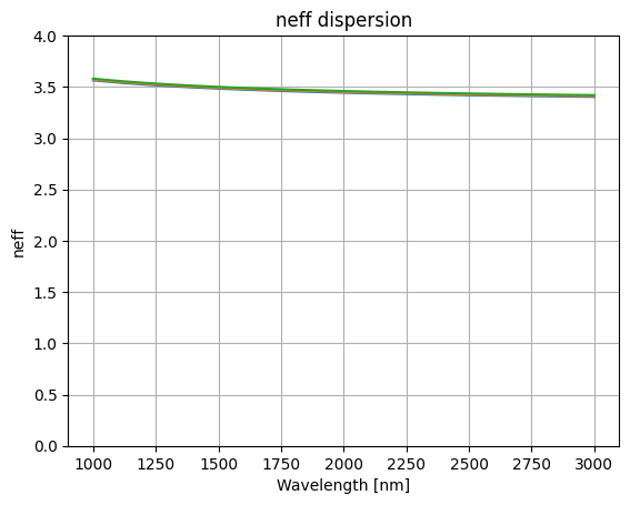
for T in [25.0, 35.0, 45.0]:
    plt.plot(1e3 * wls, silicon_index(wls, T))
plt.xlabel("Wavelength [nm]")
plt.ylabel("neff")
plt.title("neff dispersion")
plt.grid(True)
plt.ylim(0, 4)
plt.show()
Waveguide Modes
We can use meow to calculate the modes in our waveguide:
def find_waveguide_modes(
    wl: float = 1.55,
    T: float = 25.0,
    n_box: float = 1.4,
    n_clad: float = 1.4,
    n_core: float | None = None,
    t_slab: float = 0.1,
    t_soi: float = 0.22,
    w_core: float = 0.45,
    du=0.02,
    n_modes: int = 10,
    cache_path: str | Path = "modes",
    *,
    replace_cached: bool = False,
):
    length = 10.0
    delta = 10 * du
    env = mw.Environment(wl=wl, T=T)
    if n_core is None:
        n_core = silicon_index(wl, T)
    cache_path = Path(cache_path).resolve()
    cache_path.mkdir(exist_ok=True)
    fn = f"{wl=:.2f}-{T=:.2f}-{n_box=:.2f}-{n_clad=:.2f}-{n_core=:.5f}-{t_slab=:.3f}-{t_soi=:.3f}-{w_core=:.3f}-{du=:.3f}-{n_modes=}.json"
    path = cache_path / fn
    if not replace_cached and path.exists():
        return [mw.Mode.model_validate(mode) for mode in json.loads(path.read_text())]

    # fmt: off
    m_core = mw.SampledMaterial(name="slab", n=np.asarray([n_core, n_core]), params={"wl": np.asarray([1.0, 2.0])}, meta={"color": (0.9, 0, 0, 0.9)})
    m_clad = mw.SampledMaterial(name="clad", n=np.asarray([n_clad, n_clad]), params={"wl": np.asarray([1.0, 2.0])})
    m_box = mw.SampledMaterial(name="box", n=np.asarray([n_box, n_box]), params={"wl": np.asarray([1.0, 2.0])})
    box = mw.Structure(material=m_box, geometry=mw.Box(x_min=- 2 * w_core - delta, x_max= 2 * w_core + delta, y_min=- 2 * t_soi - delta, y_max=0.0, z_min=0.0, z_max=length))
    slab = mw.Structure(material=m_core, geometry=mw.Box(x_min=-2 * w_core - delta, x_max=2 * w_core + delta, y_min=0.0, y_max=t_slab, z_min=0.0, z_max=length))
    clad = mw.Structure(material=m_clad, geometry=mw.Box(x_min=-2 * w_core - delta, x_max=2 * w_core + delta, y_min=0, y_max=3 * t_soi + delta, z_min=0.0, z_max=length))
    core = mw.Structure(material=m_core, geometry=mw.Box(x_min=-w_core / 2, x_max=w_core / 2, y_min=0.0, y_max=t_soi, z_min=0.0, z_max=length))

    cell = mw.Cell(structures=[box, clad, slab, core], mesh=mw.Mesh2D( x=np.arange(-2*w_core, 2*w_core, du), y=np.arange(-2*t_soi, 3*t_soi, du) ), z_min=0.0, z_max=10.0)
    cross_section = mw.CrossSection.from_cell(cell=cell, env=env)
    modes = mw.compute_modes(cross_section, num_modes=n_modes)
    # fmt: on

    path.write_text(json.dumps([json.loads(mode.model_dump_json()) for mode in modes]))

    return modes
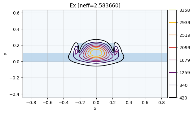
We can now easily calculate the modes of a strip waveguide:
def calculate_neffs(wls, Ts, *, replace_cached=False):
    key = md5(wls.tobytes() + b"\x00" + Ts.tobytes()).hexdigest()[:8]
    path = Path("modes").resolve() / f"{key}.csv"
    if not replace_cached and path.exists():
        return pd.read_csv(path)
    neffs = np.zeros((wls.shape[0], Ts.shape[0]))
    for i, wl in enumerate(pb := tqdm(wls)):
        for j, T in enumerate(Ts):
            pb.set_postfix(T=f"{T:.2f}C")
            modes = find_waveguide_modes(wl=wl, T=T, w_core=0.5, replace_cached=False)
            neffs[i, j] = np.real(modes[0].neff)

    xarr = xr.DataArray(data=neffs, coords={"wl": wls, "T": Ts})
    df = sax.to_df(xarr, target_name="neff")
    df.to_csv(path, index=False)
    return df
wls = np.linspace(1.0, 3.0, 21)
Ts = np.linspace(25, 35, 11)
df = calculate_neffs(wls, Ts, replace_cached=False)
0%| | 0/21 [00:00<?, ?it/s]
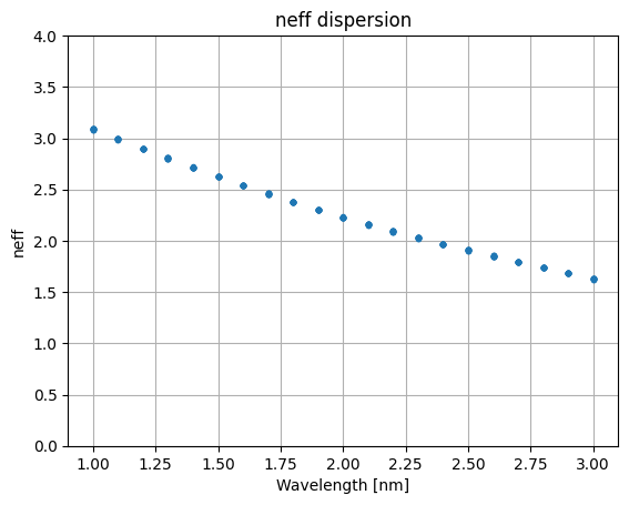
plt.plot(df.wl, df.neff, ls="none", marker=".")
plt.xlabel("Wavelength [nm]")
plt.ylabel("neff")
plt.title("neff dispersion")
plt.grid(True)
plt.ylim(0, 4)
plt.show()
result = sax.fit.neural_fit(df, targets=["neff"], num_epochs=3000)
surface_model = result["predict_fn"]
0%| | 0/3000 [00:00<?, ?it/s]
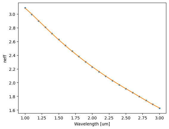
Prediction
T = 31.0
df_sel = df.query(f"T=={T:.1f}")
plt.plot(df_sel.wl, df_sel.neff, ls="none", marker=".")
wl = jnp.linspace(df_sel.wl.min(), df_sel.wl.max(), 201)
T = T * jnp.ones_like(wl)
neff_pred = surface_model(jnp.stack([wl, T], axis=1))
plt.plot(wl, neff_pred)
plt.xlabel("Wavelength [um]")
plt.ylabel("neff")
plt.show()
Equation
\(\displaystyle - 0.110410410278069 \tanh{\left(- 0.600357580564615 T + 1.54715370730798 wl + 14.2374485042365 \right)} + 0.179689236065544 \tanh{\left(- 0.457454411479906 T + 1.25572687935246 wl + 10.6201873225657 \right)} + 0.106318738569301 \tanh{\left(- 0.25623610731175 T + 1.67010379109252 wl + 5.12134080369482 \right)} - 0.089462544898889 \tanh{\left(- 0.226044694019929 T + 0.789923085868438 wl + 4.70140825870355 \right)} - 0.151499828616495 \tanh{\left(- 0.188554713201419 T + 1.59812963469096 wl + 3.23722378461125 \right)} + 0.382027195756166 \tanh{\left(0.0037683655454634 T - 1.83996384010034 wl + 1.92716523528966 \right)} + 0.17646629600736 \tanh{\left(0.0104931609250196 T - 2.29046886360609 wl + 6.25742206550521 \right)} - 0.197570742586323 \tanh{\left(0.0621753248785342 T + 1.18170050383529 wl - 4.11549409189787 \right)} + 0.410408775605637 \tanh{\left(0.0954941703146014 T - 2.12122630034377 wl + 1.30069683370671 \right)} - 0.221116759823089 \tanh{\left(0.131097472903566 T - 2.50870475465287 wl + 0.931594589044195 \right)} + 2.45595599268768\)
Python Function
def neff(
    wl: sax.FloatArrayLike,
    T: sax.FloatArrayLike,
) -> sax.FloatArray:
    return jnp.asarray(-0.110410410278069*jnp.tanh(-0.600357580564615*T + 1.54715370730798*wl + 14.2374485042365) + 0.179689236065544*jnp.tanh(-0.457454411479906*T + 1.25572687935246*wl + 10.6201873225657) + 0.106318738569301*jnp.tanh(-0.25623610731175*T + 1.67010379109252*wl + 5.12134080369482) - 0.089462544898889*jnp.tanh(-0.226044694019929*T + 0.789923085868438*wl + 4.70140825870355) - 0.151499828616495*jnp.tanh(-0.188554713201419*T + 1.59812963469096*wl + 3.23722378461125) + 0.382027195756166*jnp.tanh(0.0037683655454634*T - 1.83996384010034*wl + 1.92716523528966) + 0.17646629600736*jnp.tanh(0.0104931609250196*T - 2.29046886360609*wl + 6.25742206550521) - 0.197570742586323*jnp.tanh(0.0621753248785342*T + 1.18170050383529*wl - 4.11549409189787) + 0.410408775605637*jnp.tanh(0.0954941703146014*T - 2.12122630034377*wl + 1.30069683370671) - 0.221116759823089*jnp.tanh(0.131097472903566*T - 2.50870475465287*wl + 0.931594589044195) + 2.45595599268768)
# copied from the output above
def neff(
    wl: sax.FloatArrayLike,
    T: sax.FloatArrayLike,
) -> sax.FloatArray:
    return jnp.asarray(-0.111191802586104*jnp.tanh(-0.600317366952325*T + 1.54846504944971*wl + 14.2272048582564) + 0.180757975443552*jnp.tanh(-0.457411832080669*T + 1.25568437816402*wl + 10.614732777431) + 0.107327818114191*jnp.tanh(-0.25649703408395*T + 1.67111893010048*wl + 5.1256823674601) - 0.0898577799557729*jnp.tanh(-0.225850362933715*T + 0.790158764514527*wl + 4.69186447361556) - 0.151898347397017*jnp.tanh(-0.189879669993807*T + 1.59611170859548*wl + 3.27735371452777) + 0.383908389244572*jnp.tanh(0.00369014645440011*T - 1.83824748809467*wl + 1.93052206415554) + 0.177426903448328*jnp.tanh(0.0102029156991074*T - 2.29191621436434*wl + 6.26841403281157) - 0.198500270340145*jnp.tanh(0.061876158041826*T + 1.18462265069521*wl - 4.11404913741124) + 0.412859497897128*jnp.tanh(0.0953365220520588*T - 2.12223348019723*wl + 1.30945166982991) - 0.222415152240564*jnp.tanh(0.131198421445111*T - 2.50971948440061*wl + 0.935123955664435) + 2.46005737019216)  # fmt: skip
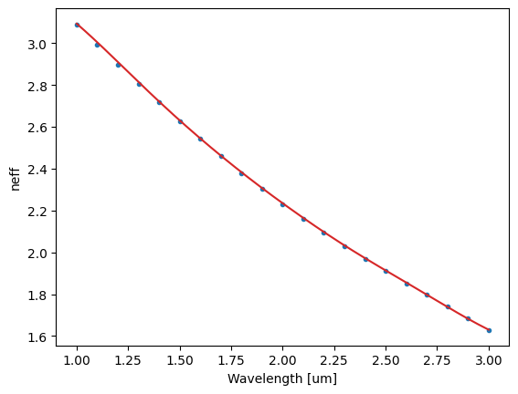
T = 31.0
df_sel = df.query(f"T=={T:.1f}")
plt.plot(df_sel.wl, df_sel.neff, ls="none", marker=".")
wl = jnp.linspace(df_sel.wl.min(), df_sel.wl.max(), 201)
T = T * jnp.ones_like(wl)
neff_pred = neff(wl, T)
plt.plot(wl, neff_pred, color="C3")
plt.xlabel("Wavelength [um]")
plt.ylabel("neff")
plt.show()