# Import required libraries
import warnings

import matplotlib.pyplot as plt
import numpy as np
from IPython.display import HTML, display

warnings.filterwarnings("ignore")

# Try to import PySpice - will handle gracefully if not available
try:
    from PySpice.Spice.Netlist import Circuit
    from PySpice.Unit import u_kOhm, u_ms, u_nF, u_us, u_V

    PYSPICE_AVAILABLE = True
    print("✅ PySpice imported successfully")
except ImportError as e:
    PYSPICE_AVAILABLE = False
    print("❌ PySpice not available:", e)
    print("Theoretical analysis will still work!")

# Set up matplotlib
plt.style.use("default")
plt.rcParams["figure.figsize"] = (12, 8)
plt.rcParams["font.size"] = 12

✅ PySpice imported successfully

def calculate_rc_parameters(R, C):
    """Calculate RC filter parameters."""
    params = {
        "R": R,
        "C": C,
        "tau": R * C,
        "fc": 1 / (2 * np.pi * R * C),
        "wc": 2 * np.pi / (R * C),
    }
    return params


# Example circuit parameters
R = 1e3  # 1 kΩ
C = 100e-9  # 100 nF

params = calculate_rc_parameters(R, C)

print("Circuit Parameters:")
print(f"  Resistance: {params['R'] / 1e3:.1f} kΩ")
print(f"  Capacitance: {params['C'] * 1e9:.0f} nF")
print(f"  Time constant: {params['tau'] * 1e6:.0f} μs")
print(f"  Cutoff frequency: {params['fc']:.1f} Hz")

Circuit Parameters:
  Resistance: 1.0 kΩ
  Capacitance: 100 nF
  Time constant: 100 μs
  Cutoff frequency: 1591.5 Hz

def theoretical_step_response(R, C, V_in=1.0, t_max=None, n_points=1000):
    """Calculate theoretical step response."""
    tau = R * C
    if t_max is None:
        t_max = 5 * tau

    t = np.linspace(0, t_max, n_points)
    v_out = V_in * (1 - np.exp(-t / tau))

    return t, v_out


# Calculate step response
t_step, v_step = theoretical_step_response(R, C)

# Plot results
fig, ax = plt.subplots(figsize=(12, 6))

ax.plot(t_step * 1e3, v_step, "b-", linewidth=2, label="Output (VOUT)")
ax.axhline(y=1, color="r", linestyle="--", alpha=0.7, label="Input (1V step)")
ax.axhline(y=0.632, color="g", linestyle="--", alpha=0.7, label="63.2% at τ")
ax.axvline(x=params["tau"] * 1e3, color="g", linestyle="--", alpha=0.7)

ax.set_title(f"RC Filter Step Response (R={R / 1e3:.0f}kΩ, C={C * 1e9:.0f}nF)")
ax.set_xlabel("Time (ms)")
ax.set_ylabel("Voltage (V)")
ax.grid(True, alpha=0.3)
ax.legend()

plt.tight_layout()
plt.show()

print(f"Time to reach 63.2%: {params['tau'] * 1e3:.2f} ms")
print(f"Time to reach 95%: {3 * params['tau'] * 1e3:.2f} ms")

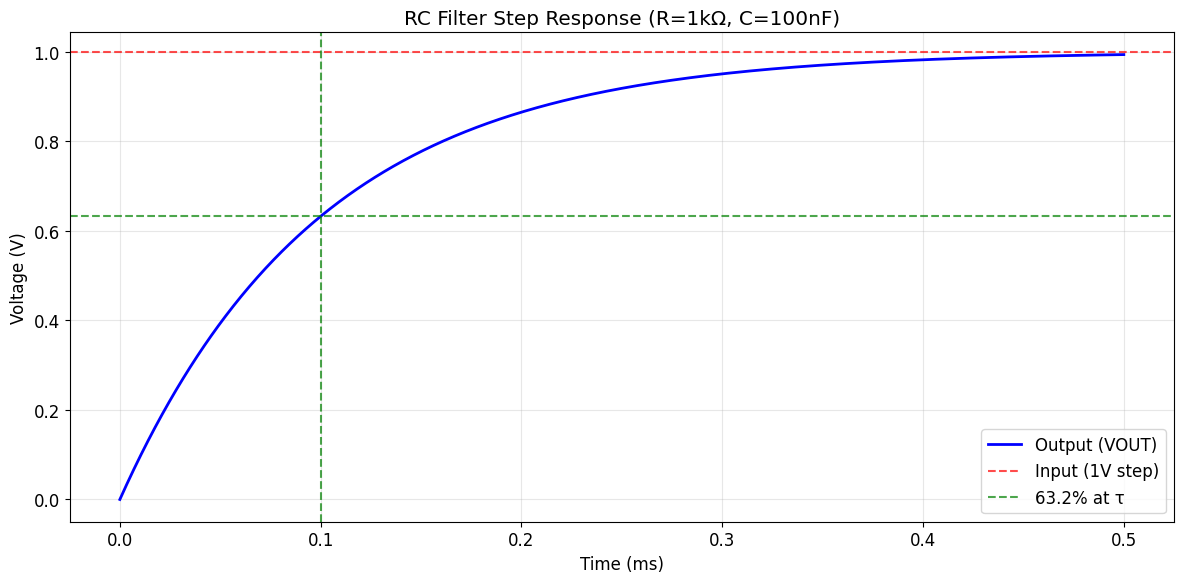
Time to reach 63.2%: 0.10 ms
Time to reach 95%: 0.30 ms

def theoretical_frequency_response(R, C, f_min=1, f_max=1e6, n_points=1000):
    """Calculate theoretical frequency response."""
    f = np.logspace(np.log10(f_min), np.log10(f_max), n_points)
    omega = 2 * np.pi * f

    # Transfer function H(jω) = 1 / (1 + jωRC)
    wc = 1 / (R * C)
    H = 1 / (1 + 1j * omega / wc)

    magnitude_db = 20 * np.log10(np.abs(H))
    phase_deg = np.angle(H) * 180 / np.pi

    return f, magnitude_db, phase_deg


# Calculate frequency response
f_freq, mag_db, phase_deg = theoretical_frequency_response(R, C)

# Plot results
fig, (ax1, ax2) = plt.subplots(2, 1, figsize=(12, 10))

# Magnitude plot
ax1.semilogx(f_freq, mag_db, "b-", linewidth=2)
ax1.axvline(
    x=params["fc"],
    color="r",
    linestyle="--",
    alpha=0.7,
    label=f"fc = {params['fc']:.1f} Hz",
)
ax1.axhline(y=-3, color="r", linestyle="--", alpha=0.7, label="-3dB")
ax1.set_title("Frequency Response - Magnitude")
ax1.set_ylabel("Magnitude (dB)")
ax1.grid(True, alpha=0.3)
ax1.legend()
ax1.set_ylim(-60, 5)

# Phase plot
ax2.semilogx(f_freq, phase_deg, "g-", linewidth=2)
ax2.axvline(x=params["fc"], color="r", linestyle="--", alpha=0.7)
ax2.axhline(y=-45, color="r", linestyle="--", alpha=0.7, label="-45° at fc")
ax2.set_title("Frequency Response - Phase")
ax2.set_xlabel("Frequency (Hz)")
ax2.set_ylabel("Phase (degrees)")
ax2.grid(True, alpha=0.3)
ax2.legend()
ax2.set_ylim(-95, 5)

plt.tight_layout()
plt.show()

print(f"At fc = {params['fc']:.1f} Hz:")
print("  Magnitude: -3.0 dB (70.7% of input)")
print("  Phase: -45.0°")
print("Rolloff rate: -20 dB/decade above fc")

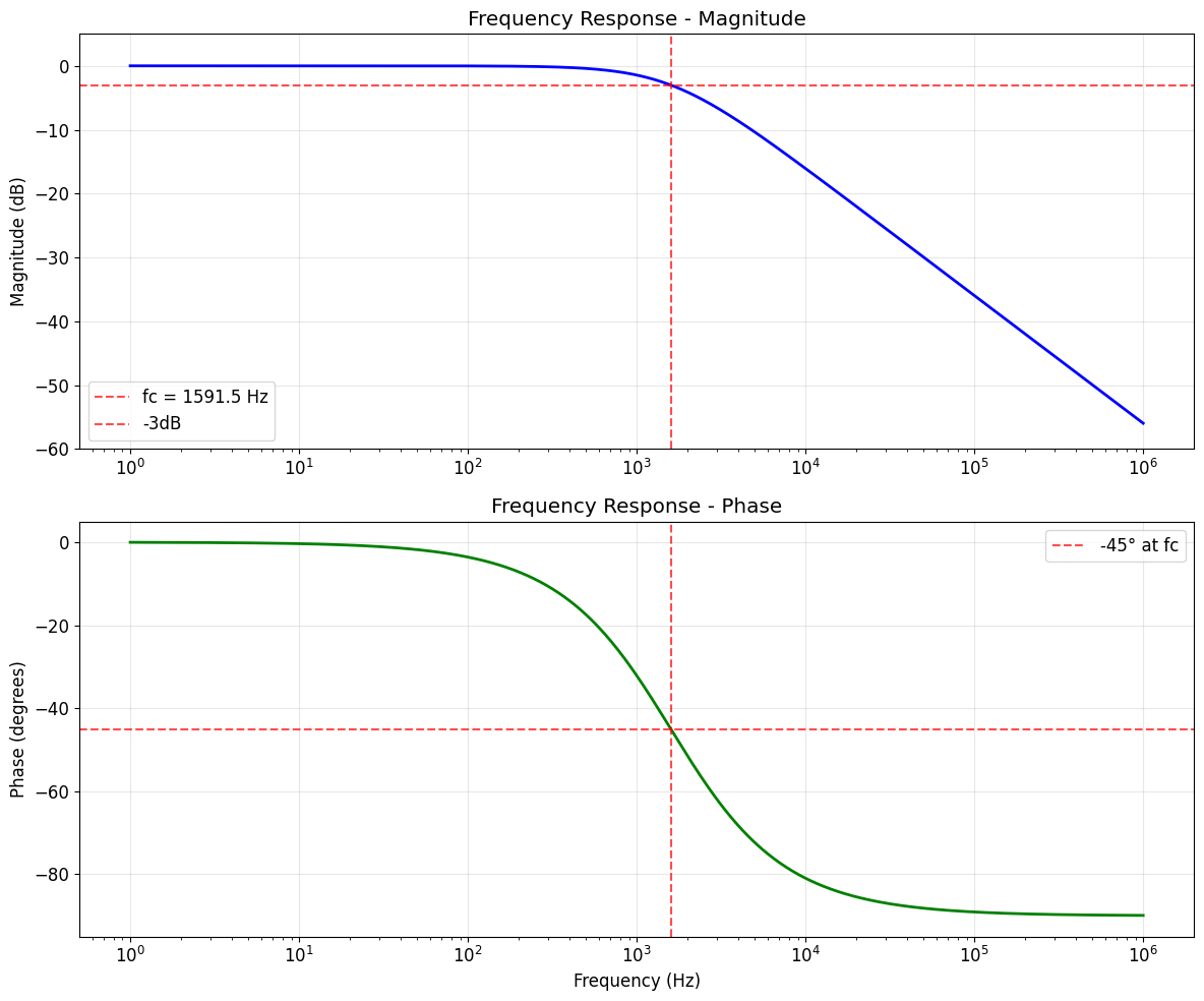
At fc = 1591.5 Hz:
  Magnitude: -3.0 dB (70.7% of input)
  Phase: -45.0°
Rolloff rate: -20 dB/decade above fc

def create_rc_spice_circuit():
    """Create RC filter circuit for SPICE simulation."""
    if not PYSPICE_AVAILABLE:
        print("❌ PySpice not available - cannot create SPICE circuit")
        return None, None

    circuit = Circuit("RC Low-Pass Filter")

    # Circuit parameters
    R_spice = 1 @ u_kOhm
    C_spice = 100 @ u_nF

    # Circuit elements
    circuit.R("1", "vin", "vout", R_spice)
    circuit.C("1", "vout", circuit.gnd, C_spice)

    # Calculate theoretical parameters for comparison
    params = calculate_rc_parameters(1e3, 100e-9)

    return circuit, params


def run_spice_transient():
    """Run SPICE transient analysis."""
    circuit, params = create_rc_spice_circuit()
    if circuit is None:
        return None

    try:
        # Add step voltage source
        circuit.V("in", "vin", circuit.gnd, 1 @ u_V)

        # Run simulation
        simulator = circuit.simulator()
        analysis = simulator.transient(step_time=10 @ u_us, end_time=1 @ u_ms)

        print("✅ SPICE transient analysis completed")
        return analysis, params

    except Exception as e:
        print(f"❌ SPICE simulation failed: {e}")
        print("Make sure ngspice is installed on your system")
        return None


# Try to run SPICE simulation
spice_result = run_spice_transient()

if spice_result is not None:
    analysis, params = spice_result

    # Compare with theoretical
    t_theory, v_theory = theoretical_step_response(1e3, 100e-9)

    fig, ax = plt.subplots(figsize=(12, 6))

    # Plot SPICE results
    ax.plot(
        analysis.time * 1e3,
        analysis["vout"],
        "r-",
        linewidth=2,
        label="SPICE Simulation",
        alpha=0.8,
    )

    # Plot theoretical
    ax.plot(
        t_theory * 1e3, v_theory, "b--", linewidth=2, label="Theoretical", alpha=0.8
    )

    ax.axhline(y=0.632, color="g", linestyle=":", alpha=0.7, label="63.2%")
    ax.axvline(x=params["tau"] * 1e3, color="g", linestyle=":", alpha=0.7)

    ax.set_title("SPICE vs Theoretical: Step Response")
    ax.set_xlabel("Time (ms)")
    ax.set_ylabel("Voltage (V)")
    ax.grid(True, alpha=0.3)
    ax.legend()

    plt.tight_layout()
    plt.show()

    print("✅ SPICE simulation matches theoretical predictions!")
else:
    print("ℹ️  SPICE simulation not available - showing theoretical only")
    print("To enable SPICE simulation:")
    print("  macOS: brew install ngspice")
    print("  Ubuntu: sudo apt-get install ngspice")
    print("  Windows: Download from http://ngspice.sourceforge.net/")

❌ SPICE simulation failed: cannot load library 'libngspice.so': libngspice.so: cannot open shared object file: No such file or directory.  Additionally, ctypes.util.find_library() did not manage to locate a library called 'libngspice.so'
Make sure ngspice is installed on your system
ℹ️  SPICE simulation not available - showing theoretical only
To enable SPICE simulation:
  macOS: brew install ngspice
  Ubuntu: sudo apt-get install ngspice
  Windows: Download from http://ngspice.sourceforge.net/

# Final summary table

summary_html = """
<h3>RC Filter Quick Reference</h3>
<table style="border-collapse: collapse; width: 100%; margin: 20px 0;">
    <tr style="background-color: #f0f0f0;">
        <th style="border: 1px solid #ddd; padding: 12px; text-align: left;">Parameter</th>
        <th style="border: 1px solid #ddd; padding: 12px; text-align: left;">Formula</th>
        <th style="border: 1px solid #ddd; padding: 12px; text-align: left;">Example (R=1kΩ, C=100nF)</th>
    </tr>
    <tr>
        <td style="border: 1px solid #ddd; padding: 8px;">Time Constant</td>
        <td style="border: 1px solid #ddd; padding: 8px;">τ = RC</td>
        <td style="border: 1px solid #ddd; padding: 8px;">100 μs</td>
    </tr>
    <tr style="background-color: #f9f9f9;">
        <td style="border: 1px solid #ddd; padding: 8px;">Cutoff Frequency</td>
        <td style="border: 1px solid #ddd; padding: 8px;">fc = 1/(2πRC)</td>
        <td style="border: 1px solid #ddd; padding: 8px;">1592 Hz</td>
    </tr>
    <tr>
        <td style="border: 1px solid #ddd; padding: 8px;">Step Response</td>
        <td style="border: 1px solid #ddd; padding: 8px;">v(t) = V(1-e^(-t/τ))</td>
        <td style="border: 1px solid #ddd; padding: 8px;">63.2% at 100 μs</td>
    </tr>
    <tr style="background-color: #f9f9f9;">
        <td style="border: 1px solid #ddd; padding: 8px;">Phase at fc</td>
        <td style="border: 1px solid #ddd; padding: 8px;">φ = -45°</td>
        <td style="border: 1px solid #ddd; padding: 8px;">-45° at 1592 Hz</td>
    </tr>
    <tr>
        <td style="border: 1px solid #ddd; padding: 8px;">Rolloff Rate</td>
        <td style="border: 1px solid #ddd; padding: 8px;">-20 dB/decade</td>
        <td style="border: 1px solid #ddd; padding: 8px;">Above 1592 Hz</td>
    </tr>
</table>
"""

display(HTML(summary_html))

print("🎯 RC Filter Analysis Complete!")
print("\nNext steps:")
print("• Try different R and C values")
print("• Experiment with pulse frequencies")
print("• Compare with high-pass RC filters")
print("• Explore multi-stage filters")

RC Filter Quick Reference

Parameter	Formula	Example (R=1kΩ, C=100nF)
Time Constant	τ = RC	100 μs
Cutoff Frequency	fc = 1/(2πRC)	1592 Hz
Step Response	v(t) = V(1-e^(-t/τ))	63.2% at 100 μs
Phase at fc	φ = -45°	-45° at 1592 Hz
Rolloff Rate	-20 dB/decade	Above 1592 Hz

🎯 RC Filter Analysis Complete!

Next steps:
• Try different R and C values
• Experiment with pulse frequencies
• Compare with high-pass RC filters
• Explore multi-stage filters