This notebook demonstrates 2D effective-index FDTD simulations using gsim.meep.

2D simulations collapse the z-dimension, making them 10–100× faster than full 3D. They use an effective-index approximation and enforce TE polarization.

When to use 2D: - Quick design-space exploration and parameter sweeps - Verifying port connectivity and mode coupling before committing to 3D - Components where vertical confinement is well-described by an effective index

Requirements:

• GDSFactory+ account for cloud simulation

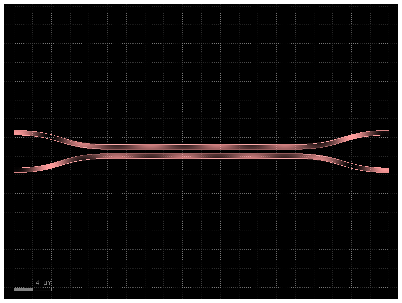
Load a pcell from UBC PDK¶

import gdsfactory as gf

gf.gpdk.PDK.activate()

c = gf.components.coupler(gap=0.5)
c

Configure 2D simulation¶

The only difference from a 3D simulation is sim.solver.is_3d = False. This collapses the z-dimension, ignores sidewall angles, and enforces TE polarization.

from gsim import meep
from gsim.common.stack import get_stack
from gsim.meep.models.api import Material

stack = get_stack()  # auto-detects active PDK

sim = meep.Simulation()

sim.geometry(component=c, stack=stack)
sim.materials = {
    "si": Material(refractive_index=3.47),
    "SiO2": Material(refractive_index=1.44),
}
sim.source(port="o1", wavelength=1.55, wavelength_span=0.01)
sim.monitors = ["o1", "o2", "o3"]
sim.domain(pml=1.0, margin=0.5)
sim.solver(resolution=25, is_3d=False)
sim.num_freqs = 21
sim.solver.stop_when_energy_decayed()

print(sim.validate_config())

Stack validation: PASSED
Warnings:
  - Stopping: energy_decay (dt=20.0, decay_by=0.01, cap=2000.0)

Preview geometry¶

sim.plot_2d(slices="z")

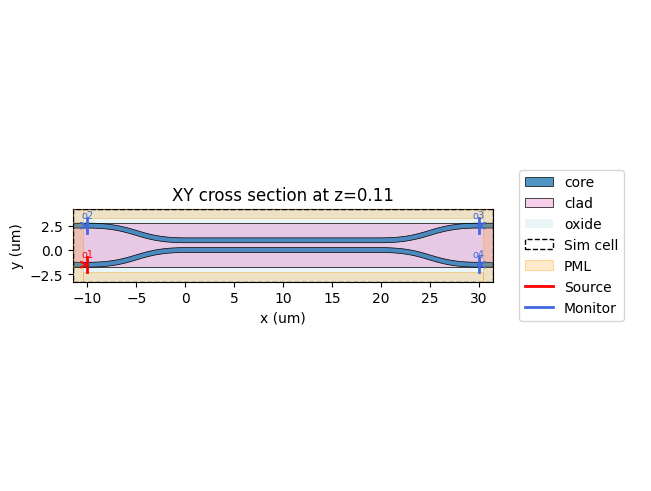
For an interactive preview, use plot_2d_interactive(). It returns a Plotly figure where you can zoom, pan, and toggle individual layers, materials, PML regions, and ports on/off via the legend.

sim.plot_2d_interactive()

Run 2D simulation on cloud¶

result = sim.run()

  meep-05064e24  completed  2m 05s


Extracting results.tar.gz...
Downloaded 4 files to sim-data-meep-05064e24

result.plot_interactive()

result.plot_interactive(phase=True)