Mode Solver — TFLN Ridge Waveguide (meep)
Fundamental TE mode of thin-film lithium niobate ridge waveguide at lambda=1.55 µm. Reference: Ying Li et al., ACS Omega 2023, 8(10), 9644–9651.
Design: SiO2 cladding / LiNbO3 slab 220 nm / LiNbO3 ridge 180 nm (total 400 nm), ridge width 1.1 µm, sidewall angle 17°.
Expected: n_eff ~ 1.85, n_group ~ 2.20.
background_material="sio2" fills unpatterned space with SiO2.
Imports
import gdsfactory as gf
import matplotlib.pyplot as plt
import numpy as np

import gsim.meep as gm
from gsim.common.stack.extractor import Layer, LayerStack

plt.close()

gf.gpdk.PDK.activate()
pyvirtualdisplay not available; continuing without Xvfb
LiNbO3 material (Zelmon 1997)
LiNbO3 is birefringent and is now registered as a uniaxial material
in gsim.common.stack.materials.MATERIALS_DB (notebook no longer
manually registers it). Both ordinary and extraordinary Sellmeier
models from Zelmon et al. (JOSA B 14(12), 3319--3322, 1997) are included:
Ordinary: n_o^2 = 1 + 2.6734 lam2/(lam2 - 0.01764) + 1.2290 lam2/(lam2 - 0.05914) + 12.614 lam2/(lam2 - 474.60)
Extraordinary: n_e^2 = 1 + 2.9804 lam2/(lam2 - 0.02047) + 0.5981 lam2/(lam2 - 0.0666) + 8.9543 lam2/(lam2 - 416.08)
For x-cut TFLN the TE mode's dominant E-field aligns with the extraordinary axis (zz).
Build the GDS component
SLAB_WIDTH = 5.0  # um --- wide slab
CORE_WIDTH = 1.1  # um --- w0 from reference design
LENGTH = 10.0  # um --- waveguide length (arbitrary for mode solving)

c = gf.Component()

# LiNbO3 ridge (layer 2) --- narrow core on top
c.add_polygon(
    [
        (-LENGTH / 2, -CORE_WIDTH / 2),
        (LENGTH / 2, -CORE_WIDTH / 2),
        (LENGTH / 2, CORE_WIDTH / 2),
        (-LENGTH / 2, CORE_WIDTH / 2),
    ],
    layer=(2, 0),
)

# Ports at both ends
c.add_port(
    name="o1",
    center=(-LENGTH / 2, 0),
    width=CORE_WIDTH,
    orientation=180,
    layer=(1, 0),
)
c.add_port(
    name="o2",
    center=(LENGTH / 2, 0),
    width=CORE_WIDTH,
    orientation=0,
    layer=(1, 0),
)

print(f"Component: {c.name}")
print(f"  Ports:  {[p.name for p in c.ports]}")
print(f"  Layers: {list(c.layers)}")
Component: Unnamed_0
  Ports:  ['o1', 'o2']
  Layers: [(2, 0)]
Layer stack
SiO2 fills background via background_material="sio2".
SLAB_THICKNESS = 0.22  # um  (h3)
CORE_THICKNESS = 0.40  # um --- total LiNbO3 thickness
RIDGE_THICKNESS = CORE_THICKNESS - SLAB_THICKNESS  # 0.18 um

layers = {
    "box": Layer(
        name="box",
        gds_layer=(0, 0),
        zmin=-1.0,
        zmax=0.0,
        thickness=1.0,
        material="sio2",
        layer_type="dielectric",
    ),
    "slab": Layer(
        name="slab",
        gds_layer=(1, 0),
        zmin=0.0,
        zmax=SLAB_THICKNESS,
        thickness=SLAB_THICKNESS,
        material="linbo3",
        layer_type="dielectric",
    ),
    "ridge": Layer(
        name="ridge",
        gds_layer=(2, 0),
        zmin=SLAB_THICKNESS,
        zmax=CORE_THICKNESS,
        thickness=RIDGE_THICKNESS,
        material="linbo3",
        layer_type="dielectric",
        sidewall_angle=17.0,
    ),
}
stack = LayerStack(layers=layers)

print("Layer stack (+ SiO2 background):")
for name, l in stack.layers.items():
    print(
        f"  {name:6s}  z=[{l.zmin:+.3f}, {l.zmax:+.3f}]  "
        f"t={l.thickness:.3f}  material={l.material}  gds={l.gds_layer}"
    )
Layer stack (+ SiO2 background):
  box     z=[-1.000, +0.000]  t=1.000  material=sio2  gds=(0, 0)
  slab    z=[+0.000, +0.220]  t=0.220  material=linbo3  gds=(1, 0)
  ridge   z=[+0.220, +0.400]  t=0.180  material=linbo3  gds=(2, 0)
Solve
WAVELENGTH = 1.55  # um
RESOLUTION = 64  # grid points per um
PML_THICKNESS = WAVELENGTH  # um

sim = gm.Simulation(
    geometry=gm.Geometry(component=c, stack=stack),
    domain=gm.Domain(
        pml=PML_THICKNESS,
        margin_z=(0.0, 0.5),
    ),
)
sim.mode_solver.wavelengths = [WAVELENGTH]
sim.mode_solver.fundamental().at_port("o1")
sim.mode_solver.y_span = SLAB_WIDTH
sim.mode_solver.n_field_y = 1000
sim.mode_solver.n_field_z = 1000
sim.mode_solver.background_material = "sio2"

sweep = sim.solve_modes(check_cache=True)
mode = sweep.at(WAVELENGTH).band(1)

print(f"n_eff     = {mode.n_eff}")
print(f"n_group   = {mode.n_group}")
print(f"kdom      = {[f'{k:.6f}' for k in mode.kdom]}")
print(f"band      = {mode.band_num}, parity = {mode.parity}")
print(f"fields    = {list(mode.fields.keys())}")
for comp, arr in mode.fields.items():
    print(f"  {comp}: shape={arr.shape}  |max|={np.abs(arr).max():.6f}")
  meep-d9c18466  completed  0m 00s


Extracting results.tar.gz...


Downloaded 10 files to sim-data-meep-d9c18466
n_eff     = 1.8600558281393749
n_group   = 2.259414906519319
kdom      = ['1.200036', '-0.000000', '0.000000']
band      = 1, parity = NO_PARITY
fields    = ['Ex', 'Ey', 'Ez', 'Hx', 'Hy', 'Hz']
  Ex: shape=(1000, 1000)  |max|=0.597531
  Ey: shape=(1000, 1000)  |max|=2.475644
  Ez: shape=(1000, 1000)  |max|=0.372790
  Hx: shape=(1000, 1000)  |max|=1.995995
  Hy: shape=(1000, 1000)  |max|=0.413430
  Hz: shape=(1000, 1000)  |max|=4.933792
Index profile
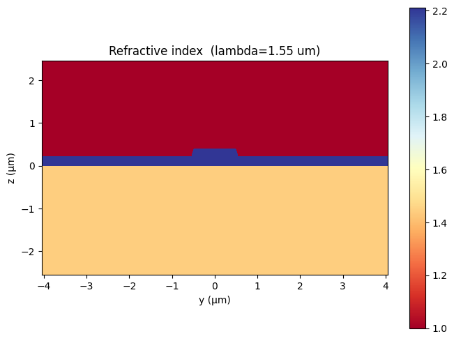
(<Figure size 700x500 with 2 Axes>,
 <Axes: title={'center': 'Refractive index  (lambda=1.55 um)'}, xlabel='y (µm)', ylabel='z (µm)'>)
Mode profile (interactive)
|field| maps for every component with zoom / pan / hover. The view is
auto-cropped to the mode region and axes use equal aspect.
import plotly.graph_objects as go
from plotly.subplots import make_subplots

comps = [c for c in ("Ex", "Ey", "Ez", "Hx", "Hy", "Hz") if c in mode.fields]

# Crop to the (small, centered) mode region and downsample so the embedded
# heatmaps stay light-weight for the docs while remaining smooth on zoom.
energy = sum(np.abs(mode.fields[c]) ** 2 for c in comps)
thr = 0.02 * energy.max()
yi = np.where(energy.max(axis=0) > thr)[0]
zi = np.where(energy.max(axis=1) > thr)[0]
dy, dz = mode.y_grid[1] - mode.y_grid[0], mode.z_grid[1] - mode.z_grid[0]
pad = 0.4  # µm margin around the mode
y0, y1 = (
    max(yi.min() - int(pad / dy), 0),
    min(yi.max() + int(pad / dy) + 1, mode.y_grid.size),
)
z0, z1 = (
    max(zi.min() - int(pad / dz), 0),
    min(zi.max() + int(pad / dz) + 1, mode.z_grid.size),
)
max_pts = 140  # per axis
sy, sz = max(1, (y1 - y0) // max_pts), max(1, (z1 - z0) // max_pts)
y_sub, z_sub = mode.y_grid[y0:y1:sy], mode.z_grid[z0:z1:sz]

fig = make_subplots(
    rows=2,
    cols=3,
    subplot_titles=[f"|{c}|" for c in comps],
    horizontal_spacing=0.08,
    vertical_spacing=0.2,
)

for i, comp in enumerate(comps):
    row, col = i // 3 + 1, i % 3 + 1
    # Mode fields are in arbitrary units; normalize each panel to its own max
    # and quantize to 8-bit (0..255). Plotly embeds arrays as binary, so this
    # keeps the notebook small while staying visually identical.
    panel = np.abs(mode.fields[comp][z0:z1:sz, y0:y1:sy])
    panel = np.round(panel / panel.max() * 255).astype(np.uint8)
    fig.add_trace(
        go.Heatmap(
            x=y_sub,
            y=z_sub,
            z=panel,
            colorscale="Inferno",
            showscale=False,
            zmin=0,
            zmax=255,
            hovertemplate=(
                "y=%{x:.3f} µm<br>z=%{y:.3f} µm<br>"
                "|" + comp + "| (rel.)=%{z}<extra></extra>"
            ),
        ),
        row=row,
        col=col,
    )
    x_anchor = "x" if i == 0 else f"x{i + 1}"
    fig.update_xaxes(title_text="y (µm)", row=row, col=col)
    fig.update_yaxes(
        title_text="z (µm)", scaleanchor=x_anchor, scaleratio=1, row=row, col=col
    )

fig.update_layout(
    height=650,
    autosize=True,
    margin=dict(t=70, b=60),
    title=dict(
        text=(
            f"lambda={WAVELENGTH:.2f} µm, w0={CORE_WIDTH:.1f} µm, "
            f"n_eff={mode.n_eff:.4f}"
        ),
        x=0.5,
        xanchor="center",
        font=dict(size=13),
    ),
)
fig.show(config={"responsive": True})
Width sweep — band diagram
Sweep the ridge width w0 and track n_eff of the first few bands.
Narrow ridges guide fewer modes, so higher-band curves appear only once the
width is wide enough to support them. Modes below the SiO2 cladding index are
radiative and are dropped (dashed line = cladding cutoff).
Each width is an independent cloud mode-solve. Jobs are submitted in batches
(up to MAX_CONCURRENT in flight) and waited on concurrently, so the whole
sweep finishes in a few minutes rather than running one width at a time.
import shutil
import tempfile
from pathlib import Path

from gsim import gcloud
from gsim.common.stack.materials import resolve_material_at_wavelength

# Snap widths to the 0.002 µm grid so gdsfactory ports stay grid-aligned.
W0_VALUES = np.round(np.linspace(0.3, 3.0, 25) / 0.002) * 0.002  # um
N_SWEEP_BANDS = 8
MAX_CONCURRENT = 10  # cloud jobs in flight at once

# SiO2 cladding index at this wavelength — guided modes must lie above it.
_clad = resolve_material_at_wavelength("sio2", WAVELENGTH)
_eps = _clad.permittivity
n_clad = float(np.sqrt(_eps if np.isscalar(_eps) else np.mean(_eps)))


def tfln_component(core_width: float) -> gf.Component:
    """Build the TFLN ridge component for a given ridge width."""
    comp = gf.Component()
    comp.add_polygon(
        [
            (-LENGTH / 2, -core_width / 2),
            (LENGTH / 2, -core_width / 2),
            (LENGTH / 2, core_width / 2),
            (-LENGTH / 2, core_width / 2),
        ],
        layer=(2, 0),
    )
    comp.add_port(
        name="o1",
        center=(-LENGTH / 2, 0),
        width=core_width,
        orientation=180,
        layer=(1, 0),
    )
    comp.add_port(
        name="o2",
        center=(LENGTH / 2, 0),
        width=core_width,
        orientation=0,
        layer=(1, 0),
    )
    return comp


def submit_mode_solve(core_width: float) -> str:
    """Upload + start one cloud mode-solve job (non-blocking). Returns job_id."""
    sim = gm.Simulation(
        geometry=gm.Geometry(component=tfln_component(core_width), stack=stack),
        domain=gm.Domain(pml=PML_THICKNESS, margin_z=(0.0, 0.5)),
    )
    sim.mode_solver.wavelengths = [WAVELENGTH]
    sim.mode_solver.first(N_SWEEP_BANDS).at_port("o1")
    sim.mode_solver.y_span = SLAB_WIDTH
    sim.mode_solver.background_material = "sio2"  # n_field=0 -> n_eff only

    tmp = Path(tempfile.mkdtemp(prefix="meep_mode_sweep_"))
    try:
        sim.write_mode_solver_config(tmp)
        input_hash, cached_job_id = gcloud.check_cache_for_dir(tmp, "meep")
        if cached_job_id is not None:
            return cached_job_id
        job_id = gcloud.upload(tmp, "meep", verbose=False, input_hash=input_hash)
        gcloud.start(job_id, verbose=False)
        return job_id
    finally:
        shutil.rmtree(tmp, ignore_errors=True)


# Submit jobs in batches so at most MAX_CONCURRENT run on the cloud at once,
# then wait for the whole batch concurrently. n_eff only (no field download).
sweep_results = []  # ModeSweepResult per width, in W0_VALUES order
for i in range(0, len(W0_VALUES), MAX_CONCURRENT):
    batch = W0_VALUES[i : i + MAX_CONCURRENT]
    job_ids = [submit_mode_solve(w0) for w0 in batch]
    print(f"batch {i // MAX_CONCURRENT + 1}: started {len(job_ids)} jobs")
    batch_results = gcloud.wait_for_results(job_ids, verbose="quiet")
    if not isinstance(batch_results, list):  # single-job batch returns one result
        batch_results = [batch_results]
    sweep_results.extend(batch_results)

# n_eff per band across the width sweep (NaN where the band is not guided).
neff_by_band = {b: [] for b in range(1, N_SWEEP_BANDS + 1)}
for w0, res in zip(W0_VALUES, sweep_results, strict=True):
    found = {r.band_num: r.n_eff for r in res.at(WAVELENGTH).results}
    for b in range(1, N_SWEEP_BANDS + 1):
        neff = found.get(b, np.nan)
        # drop radiative modes below the cladding index
        neff_by_band[b].append(neff if neff > n_clad else np.nan)
    guided = [b for b in range(1, N_SWEEP_BANDS + 1) if found.get(b, 0) > n_clad]
    summary = ", ".join(f"b{b}={found[b]:.4f}" for b in guided)
    print(f"w0={w0:.2f} µm -> {len(guided)} guided mode(s): {summary}")
4065926982.py:61: FutureWarning: Use of domain.margin_z is deprecated and will be removed in a future release; replace it with domain.z_bounds=(-1.0, 0.9).
  sim.write_mode_solver_config(tmp)


batch 1: started 10 jobs


Extracting results.tar.gz...


Extracting results.tar.gz...


Extracting results.tar.gz...


Extracting results.tar.gz...


Extracting results.tar.gz...


Extracting results.tar.gz...


Extracting results.tar.gz...


Extracting results.tar.gz...


Extracting results.tar.gz...


Extracting results.tar.gz...


batch 2: started 10 jobs


Extracting results.tar.gz...


Extracting results.tar.gz...


Extracting results.tar.gz...


Extracting results.tar.gz...


Extracting results.tar.gz...


Extracting results.tar.gz...


Extracting results.tar.gz...


Extracting results.tar.gz...


Extracting results.tar.gz...


Extracting results.tar.gz...


batch 3: started 5 jobs


Extracting results.tar.gz...


Extracting results.tar.gz...


Extracting results.tar.gz...


Extracting results.tar.gz...


Extracting results.tar.gz...
w0=0.30 µm -> 8 guided mode(s): b1=1.7447, b2=1.7259, b3=1.7129, b4=1.7262, b5=1.7211, b6=1.7270, b7=1.7201, b8=1.5921
w0=0.41 µm -> 8 guided mode(s): b1=1.7635, b2=1.7142, b3=1.7141, b4=1.7270, b5=1.7233, b6=1.7298, b7=1.7226, b8=1.6149
w0=0.52 µm -> 8 guided mode(s): b1=1.7816, b2=1.7147, b3=1.7146, b4=1.7281, b5=1.7246, b6=1.6424, b7=1.7256, b8=1.7243
w0=0.64 µm -> 8 guided mode(s): b1=1.8026, b2=1.7150, b3=1.7150, b4=1.7303, b5=1.6933, b6=1.6598, b7=1.7297, b8=1.7257
w0=0.75 µm -> 8 guided mode(s): b1=1.8210, b2=1.7152, b3=1.7152, b4=1.7343, b5=1.6938, b6=1.6734, b7=1.7336, b8=1.7266
w0=0.86 µm -> 8 guided mode(s): b1=1.8361, b2=1.7302, b3=1.7153, b4=1.7404, b5=1.6941, b6=1.7257, b7=1.7384, b8=1.7272
w0=0.98 µm -> 8 guided mode(s): b1=1.8489, b2=1.7347, b3=1.7153, b4=1.7147, b5=1.7331, b6=1.6944, b7=1.7433, b8=1.7279
w0=1.09 µm -> 8 guided mode(s): b1=1.8581, b2=1.7407, b3=1.7154, b4=1.7190, b5=1.7398, b6=1.6948, b7=1.7471, b8=1.7288
w0=1.20 µm -> 8 guided mode(s): b1=1.8671, b2=1.7509, b3=1.7155, b4=1.7237, b5=1.7455, b6=1.6953, b7=1.7504, b8=1.7302
w0=1.31 µm -> 8 guided mode(s): b1=1.8744, b2=1.7635, b3=1.7157, b4=1.7157, b5=1.7166, b6=1.6961, b7=1.7525, b8=1.7325
w0=1.42 µm -> 8 guided mode(s): b1=1.8804, b2=1.8069, b3=1.7160, b4=1.7160, b5=1.7179, b6=1.6975, b7=1.7538, b8=1.7359
w0=1.54 µm -> 8 guided mode(s): b1=1.8855, b2=1.8198, b3=1.7166, b4=1.7166, b5=1.7185, b6=1.6998, b7=1.7546, b8=1.6869
w0=1.65 µm -> 8 guided mode(s): b1=1.8894, b2=1.8302, b3=1.7174, b4=1.7173, b5=1.7188, b6=1.7024, b7=1.7552, b8=1.6914
w0=1.76 µm -> 8 guided mode(s): b1=1.8932, b2=1.8417, b3=1.7191, b4=1.7191, b5=1.7190, b6=1.7065, b7=1.7027, b8=1.6971
w0=1.88 µm -> 8 guided mode(s): b1=1.8965, b2=1.8523, b3=1.7225, b4=1.7225, b5=1.7192, b6=1.7112, b7=1.7034, b8=1.7027
w0=1.99 µm -> 8 guided mode(s): b1=1.8992, b2=1.8615, b3=1.7286, b4=1.7286, b5=1.7193, b6=1.7041, b7=1.7089, b8=1.7043
w0=2.10 µm -> 8 guided mode(s): b1=1.9016, b2=1.8698, b3=1.7369, b4=1.7369, b5=1.7196, b6=1.7063, b7=1.7158, b8=1.7059
w0=2.21 µm -> 8 guided mode(s): b1=1.9035, b2=1.8764, b3=1.7449, b4=1.7450, b5=1.7199, b6=1.7073, b7=1.7225, b8=1.7077
w0=2.32 µm -> 8 guided mode(s): b1=1.9054, b2=1.8833, b3=1.7552, b4=1.7482, b5=1.7206, b6=1.7080, b7=1.7292, b8=1.7109
w0=2.44 µm -> 8 guided mode(s): b1=1.9071, b2=1.8895, b3=1.8568, b4=1.7498, b5=1.7217, b6=1.7084, b7=1.7354, b8=1.7151
w0=2.55 µm -> 8 guided mode(s): b1=1.9085, b2=1.8949, b3=1.8662, b4=1.7512, b5=1.7237, b6=1.7086, b7=1.7406, b8=1.7200
w0=2.66 µm -> 8 guided mode(s): b1=1.9098, b2=1.8997, b3=1.8750, b4=1.7524, b5=1.7267, b6=1.7088, b7=1.7453, b8=1.7249
w0=2.78 µm -> 8 guided mode(s): b1=1.9109, b2=1.9037, b3=1.8822, b4=1.7535, b5=1.7305, b6=1.7089, b7=1.7495, b8=1.7285
w0=2.89 µm -> 8 guided mode(s): b1=1.9120, b2=1.9078, b3=1.8901, b4=1.7545, b5=1.7366, b6=1.7538, b7=1.7089, b8=1.7318
w0=3.00 µm -> 8 guided mode(s): b1=1.9129, b2=1.9115, b3=1.8975, b4=1.7555, b5=1.7439, b6=1.7573, b7=1.7092, b8=1.7339
n_eff vs w0 for each band (interactive).
band_fig = go.Figure()
for b in range(1, N_SWEEP_BANDS + 1):
    band_fig.add_trace(
        go.Scatter(
            x=W0_VALUES,
            y=neff_by_band[b],
            mode="lines+markers",
            name=f"band {b}",
            connectgaps=False,
            hovertemplate="w0=%{x:.2f} µm<br>n_eff=%{y:.4f}<extra>band "
            + str(b)
            + "</extra>",
        )
    )
band_fig.add_hline(
    y=n_clad,
    line_dash="dash",
    line_color="gray",
    annotation_text=f"SiO2 cladding (n={n_clad:.3f})",
    annotation_position="bottom right",
)
band_fig.update_layout(
    height=550,
    width=550,
    autosize=False,
    margin=dict(t=60, b=60),
    xaxis_title="ridge width w0 (µm)",
    yaxis_title="n_eff",
    title=dict(
        text=f"TFLN band diagram (lambda={WAVELENGTH:.2f} µm)",
        x=0.5,
        xanchor="center",
        font=dict(size=13),
    ),
    legend=dict(title=""),
)
# Fixed square aspect (width == height); no responsive stretch.
band_fig.show()