Propagate Modes

Propagate a modal excitation through a stack of cells using the simplified propagate_modes API

```python import matplotlib.pyplot as plt import numpy as np

import meow as mw ```

1. Structure

We use a short linear taper so the field profile evolves along z.

```python def create_structures(length=10.0, input_width=0.45, output_width=1.0): oxide = mw.Structure( material=mw.silicon_oxide, geometry=mw.Prism( poly=np.array([(0, -2.1), (length, -2.1), (length, 2.1), (0, 2.1)]), h_min=-3.0, h_max=0.0, axis="y", ), )

core = mw.Structure(
    material=mw.silicon,
    geometry=mw.Prism(
        poly=np.array(
            [
                (0, -input_width / 2),
                (length, -output_width / 2),
                (length, output_width / 2),
                (0, input_width / 2),
            ]
        ),
        h_min=0.0,
        h_max=0.22,
        axis="y",
    ),
)

return [oxide, core]

structures = create_structures() mw.visualize(structures) ```

2. Cells And Modes

The only required inputs to mw.propagate_modes are:

• modes: one mode set per cell
• cells: the corresponding EME cells

```python length = 10.0 num_cells = 8

cells = mw.create_cells( structures=structures, mesh=mw.Mesh2D( x=np.linspace(-2.0, 2.0, 121), y=np.linspace(-2.0, 2.0, 121), ), Ls=np.full(num_cells, length / num_cells), )

env = mw.Environment(wl=1.55, T=25.0) cross_sections = [mw.CrossSection.from_cell(cell=cell, env=env) for cell in cells] modes = [mw.compute_modes(cs, num_modes=4) for cs in cross_sections]

print(f"Computed {len(modes)} mode sets with {len(modes[0])} modes in the first cell.") ```

Computed 8 mode sets with 4 modes in the first cell.

3. Propagate A Fundamental Excitation

By default, mw.propagate_modes excites left mode 0 with unit amplitude and applies no right-side excitation. Here we only pass z and y so the returned field can be plotted on a known grid.

```python z = np.linspace(cells[0].z_min, cells[-1].z_max, 500) y = 0.0

field, x = mw.propagate_modes(modes, cells, y=y, z=z) print(field.shape, x.shape) ```

(500, 120) (120,)

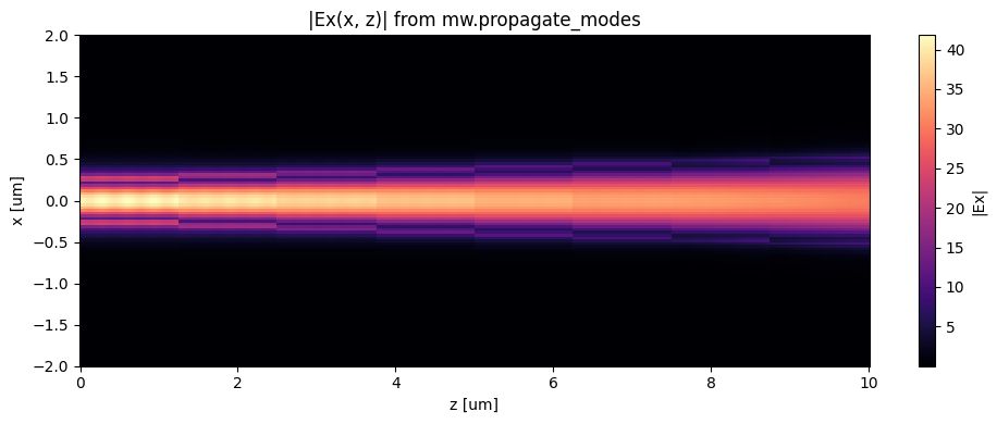
4. Plot The Reconstructed Field Slice

The returned array is an Ex(z, x) slice through the device.

python fig, ax = plt.subplots(figsize=(10, 4)) im = ax.pcolormesh(z, x, np.abs(field).T, shading="auto", cmap="magma") ax.set_xlabel("z [um]") ax.set_ylabel("x [um]") ax.set_title("|Ex(x, z)| from mw.propagate_modes") plt.colorbar(im, ax=ax, label="|Ex|") plt.tight_layout()