MZI filter#
In this example we will go over a Mach–Zehnder interferometer filter design.
Calculations#
import gdsfactory as gf
import numpy as np
def mzi(
wl: np.ndarray,
neff: float | None,
neff1: float | None = None,
neff2: float | None = None,
delta_length: float | None = None,
length1: float | None = 0,
length2: float | None = None,
) -> np.ndarray:
"""Returns Frequency Domain Response of an MZI interferometer in linear units.
Args:
wl: wavelength in um.
neff: effective index.
neff1: effective index branch 1.
neff2: effective index branch 2.
delta_length: length difference L2-L1.
length1: length of branch 1.
length2: length of branch 2.
"""
k_0 = 2 * np.pi / wl
length2 = length2 or length1 + delta_length
delta_length = delta_length or np.abs(length2 - length1)
neff1 = neff1 or neff
neff2 = neff2 or neff
E_out = 0.5 * (
np.exp(1j * k_0 * neff1 * (length1 + delta_length))
+ np.exp(1j * k_0 * neff2 * length1)
)
return np.abs(E_out) ** 2
if __name__ == "__main__":
import gplugins.tidy3d as gt
import matplotlib.pyplot as plt
nm = 1e-3
strip = gt.modes.Waveguide(
wavelength=1.55,
core_width=500 * nm,
core_thickness=220 * nm,
slab_thickness=0.0,
core_material="si",
clad_material="sio2",
)
neff = 2.46 # Effective index of the waveguides
wl0 = 1.55 # [μm] the wavelength at which neff and ng are defined
wl = np.linspace(1.5, 1.6, 1000) # [μm] Wavelengths to sweep over
ngs = [4.182551, 4.169563, 4.172917]
thicknesses = [210, 220, 230]
length = 4e3
dn = np.pi / length
polyfit_TE1550SOI_220nm = np.array(
[
1.02478963e-09,
-8.65556534e-08,
3.32415694e-06,
-7.68408985e-05,
1.19282177e-03,
-1.31366332e-02,
1.05721429e-01,
-6.31057637e-01,
2.80689677e00,
-9.26867694e00,
2.24535191e01,
-3.90664800e01,
4.71899278e01,
-3.74726005e01,
1.77381560e01,
-1.12666286e00,
]
)
def neff_w(w):
return np.poly1d(polyfit_TE1550SOI_220nm)(w)
w0 = 450 * nm
dn1 = neff_w(w0 + 1 * nm / 2) - neff_w(w0 - 1 * nm / 2)
dn5 = neff_w(w0 + 5 * nm / 2) - neff_w(w0 - 5 * nm / 2)
dn10 = neff_w(w0 + 10 * nm / 2) - neff_w(w0 - 10 * nm / 2)
pi_length1 = np.pi / dn1
pi_length5 = np.pi / dn5
pi_length10 = np.pi / dn10
print(f"pi_length = {pi_length1:.0f}um for 1nm width variation")
print(f"pi_length = {pi_length5:.0f}um for 5nm width variation")
print(f"pi_length = {pi_length10:.0f}um for 10nm width variation")
dn = dn1
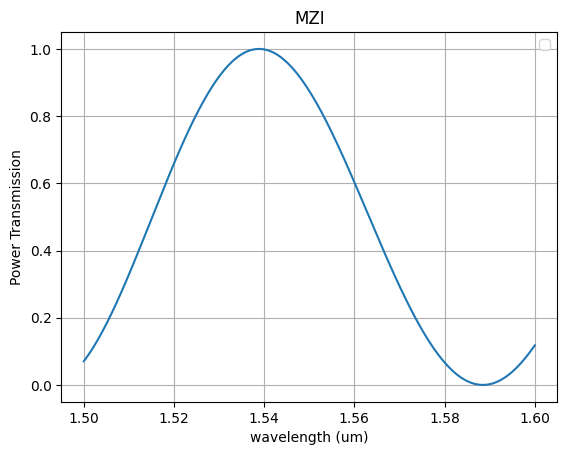
p = mzi(wl, neff=neff, neff1=neff + dn, neff2=neff + dn, delta_length=10)
plt.plot(wl, p)
plt.title("MZI")
plt.xlabel("wavelength (um)")
plt.ylabel("Power Transmission")
plt.grid()
plt.legend()
plt.show()
pi_length = 1452um for 1nm width variation
pi_length = 290um for 5nm width variation
pi_length = 145um for 10nm width variation
/tmp/ipykernel_3678/987988421.py:101: UserWarning: No artists with labels found to put in legend.  Note that artists whose label start with an underscore are ignored when legend() is called with no argument.
  plt.legend()
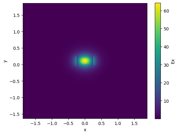
Mode solver#
For waveguides you can compute the EM modes.
import gplugins.tidy3d as gt
import matplotlib.pyplot as plt
import numpy as np

nm = 1e-3
strip = gt.modes.Waveguide(
    wavelength=1.55,
    core_width=0.5,
    core_thickness=0.22,
    slab_thickness=0.0,
    core_material="si",
    clad_material="sio2",
    group_index_step=10 * nm,
)
strip.plot_field(field_name="Ex", mode_index=0)  # TE
<matplotlib.collections.QuadMesh at 0x7f17a9e4d810>
ng = strip.n_group[0]
ng
4.178039693572359
FDTD#
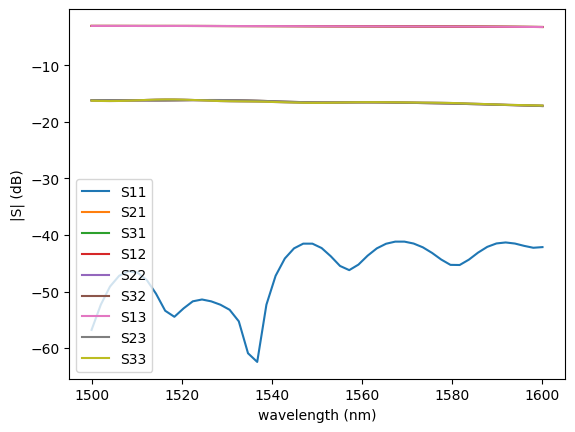
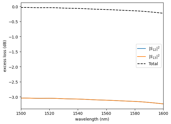
Lets compute the Sparameters of a 1x2 power splitter using tidy3D, which is a fast GPU based FDTD commercial solver.
To run, you need to create an account and add credits. The number of credits that each simulation takes depends on the simulation computation time.

import gdsfactory.components as pdk
import gplugins as sim
import gplugins.tidy3d as gt
c = pdk.mmi1x2()
c.plot()
sp = gt.write_sparameters(c, filepath="./mmi1x2.npz")
01:04:47 UTC WARNING: 'simulation.structures[0]' is outside of the simulation
             domain.
             WARNING: 'simulation.structures[0]' is outside of the simulation
             domain.
Simulation loaded from PosixPath('mmi1x2.npz')
sim.plot.plot_sparameters(sp)
sim.plot.plot_loss1x2(sp)
Circuit simulation#
For the simulations you need to build Sparameters models for your components using FDTD or other methods.

Sparameters are common in RF and photonic simulation.
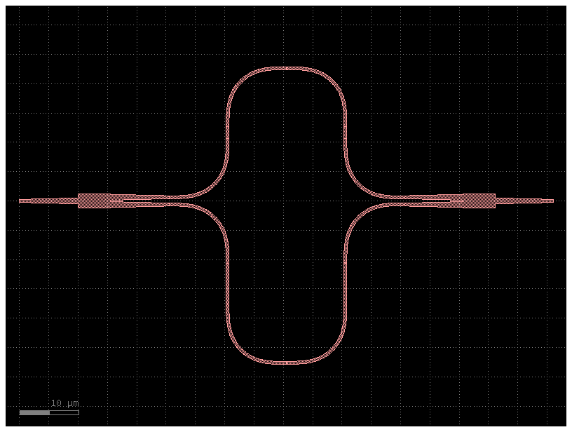
We are going to simulate a MZI interferometer circuit. For that we need to simulate each of the component Sparameters in tidy3d and then SAX Sparameter circuit solver to solve the Sparameters for the circuit. We will be using SAX which is an open source circuit simulator.
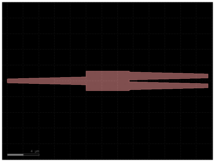
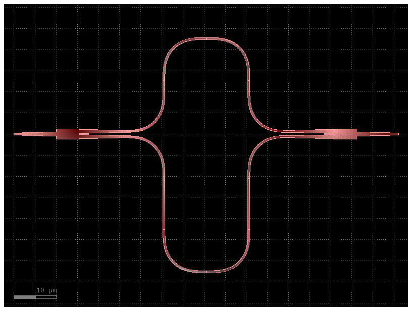
mzi10 = gf.components.mzi(splitter=c, delta_length=10)
mzi10.plot()
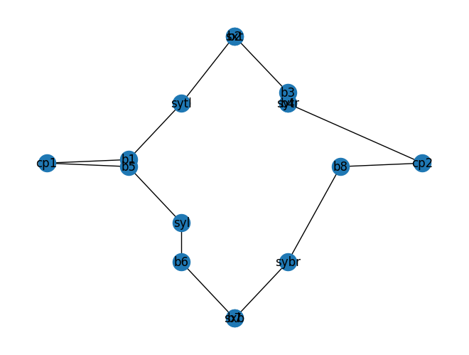
mzi10.plot_netlist()
<networkx.classes.graph.Graph at 0x7f17cdd49e10>
import gdsfactory as gf
import gplugins.sax as gsax
import jax.numpy as jnp
import matplotlib.pyplot as plt
import numpy as np
import sax
/home/runner/work/gdsfactory-photonics-training/gdsfactory-photonics-training/.venv/lib/python3.11/site-packages/sax/backends/__init__.py:58: UserWarning: klujax not found. Please install klujax for better performance during circuit evaluation!
  warnings.warn(
def straight(wl=1.5, length=10.0, neff=2.4) -> sax.SDict:
    return sax.reciprocal({("o1", "o2"): jnp.exp(2j * jnp.pi * neff * length / wl)})


def bend_euler(wl=1.5, length=20.0):
    """Assumes a reduced transmission for the euler bend compared to a straight"""
    return {k: 0.99 * v for k, v in straight(wl=wl, length=length).items()}
mmi1x2 = gsax.read.model_from_npz(sp)
models = {
    "bend_euler": bend_euler,
    "mmi1x2": mmi1x2,
    "straight": straight,
}
netlist = mzi10.get_netlist()
circuit, _ = sax.circuit(netlist=netlist, models=models)
wl = np.linspace(1.5, 1.6)
S = circuit(wl=wl)
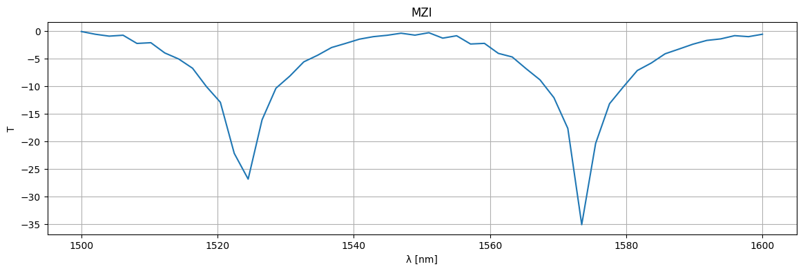
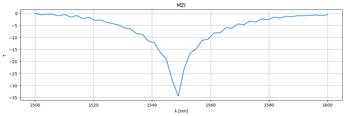
plt.figure(figsize=(14, 4))
plt.title("MZI")
plt.plot(1e3 * wl, 10 * np.log10(jnp.abs(S["o1", "o2"]) ** 2))
plt.xlabel("λ [nm]")
plt.ylabel("T")
plt.grid(True)
plt.show()
mzi20 = gf.components.mzi(splitter=c, delta_length=20)
mzi20.plot()
netlist = mzi20.get_netlist()
circuit, _ = sax.circuit(netlist=netlist, models=models)
wl = np.linspace(1.5, 1.6)
S = circuit(wl=wl)
plt.figure(figsize=(14, 4))
plt.title("MZI")
plt.plot(1e3 * wl, 10 * np.log10(jnp.abs(S["o1", "o2"]) ** 2))
plt.xlabel("λ [nm]")
plt.ylabel("T")
plt.grid(True)
plt.show()