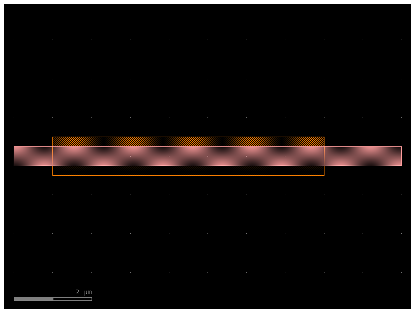
Path and CrossSection
You can create a Path in gdsfactory and extrude it with an arbitrary CrossSection.
Let us create a path:
- Create a blank
Path. - Append points to the
Pathby either using the built-in functions (arc(),straight(),euler()...) or by providing your own lists of points. - Specify
CrossSectionwith layers and offsets. - Extrude
Pathwith aCrossSectionto create a Component with the path polygons in it.
import matplotlib.pyplot as plt
import numpy as np

import gdsfactory as gf

gf.gpdk.PDK.activate()
gf.clear_cache()
Path
The first step is to generate the list of points we want the path to follow.
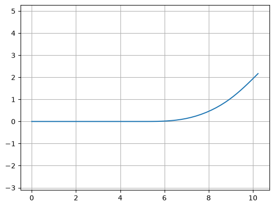
Let us now start out by creating a blank Path and using the built-in functions to
make a few smooth turns.
p1 = gf.path.straight(length=5)

# This creates a curved path segment using an Euler bend profile,
# which is a curve with a continuously changing radius designed to minimize light loss. This specific bend turns by 45 degrees.
# By setting use_eff=False, you are telling the function to ignore complex calculations and instead create a simpler bend with a constant, user-specified radius.
p2 = gf.path.euler(radius=5, angle=45, p=0.5, use_eff=False)

# The + operator is used to concatenate the two paths.
# It takes the second path (p2) and appends it to the end of the first path (p1), ensuring a smooth, continuous transition.
p = p1 + p2
p.plot()
p1 = gf.path.straight(length=5)
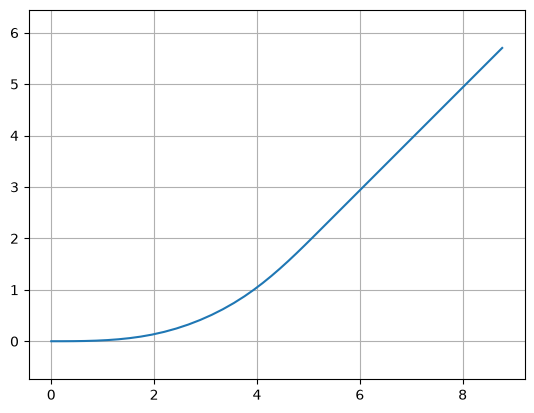
p2 = gf.path.euler(radius=5, angle=45, p=0.5, use_eff=False)
p = p2 + p1
p.plot()
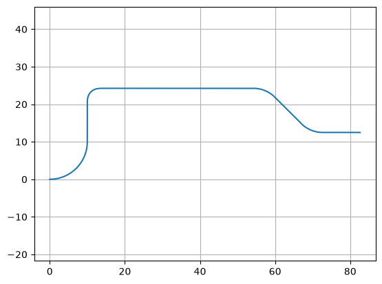
# Note: -angle rotations correspond to a clockwise turn.
P = gf.Path()
P += gf.path.arc(radius=10, angle=90)  # Circular arc.
P += gf.path.straight(length=10)  # Straight section.
P += gf.path.euler(radius=3, angle=-90)  # Euler bend (aka "racetrack" curve).
P += gf.path.straight(length=40)
P += gf.path.arc(radius=8, angle=-45)
P += gf.path.straight(length=10)
P += gf.path.arc(radius=8, angle=45)
P += gf.path.straight(length=10)

P.plot()
p2 = P.copy().rotate(45)
p2.plot()
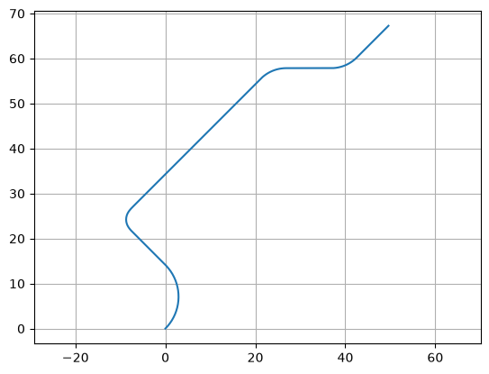
P.points - p2.points
array([[  0.        ,   0.        ],
       [  0.07775818,  -0.18109421],
       [  0.16015338,  -0.36012627],
       [  0.24713097,  -0.53697746],
       [  0.33863327,  -0.71153054],
       [  0.43459961,  -0.88366975],
       [  0.53496636,  -1.05328096],
       [  0.63966697,  -1.2202517 ],
       [  0.74863202,  -1.38447127],
       [  0.86178925,  -1.54583076],
       [  0.97906364,  -1.7042232 ],
       [  1.10037742,  -1.85954356],
       [  1.22565016,  -2.01168884],
       [  1.35479879,  -2.16055818],
       [  1.48773767,  -2.30605285],
       [  1.62437867,  -2.44807638],
       [  1.76463118,  -2.58653461],
       [  1.9084022 ,  -2.72133573],
       [  2.0555964 ,  -2.85239035],
       [  2.20611618,  -2.97961158],
       [  2.35986175,  -3.10291506],
       [  2.51673115,  -3.22221903],
       [  2.67662037,  -3.33744439],
       [  2.83942339,  -3.44851474],
       [  3.00503227,  -3.55535642],
       [  3.1733372 ,  -3.6578986 ],
       [  3.34422657,  -3.75607328],
       [  3.51758709,  -3.84981537],
       [  3.69330379,  -3.93906271],
       [  3.87126017,  -4.02375613],
       [  4.05133823,  -4.10383946],
       [  4.23341856,  -4.1792596 ],
       [  4.41738044,  -4.24996655],
       [  4.60310189,  -4.31591343],
       [  4.79045976,  -4.3770565 ],
       [  4.97932982,  -4.43335522],
       [  5.16958684,  -4.48477228],
       [  5.36110467,  -4.53127356],
       [  5.55375631,  -4.57282824],
       [  5.74741403,  -4.60940877],
       [  5.94194941,  -4.64099089],
       [  6.13723348,  -4.66755366],
       [  6.33313674,  -4.68907946],
       [  6.52952929,  -4.70555403],
       [  6.72628092,  -4.71696644],
       [  6.92326117,  -4.72330911],
       [  7.12033942,  -4.72457786],
       [  7.317385  ,  -4.72077183],
       [  7.51426725,  -4.71189355],
       [  7.71085564,  -4.69794891],
       [  7.90701981,  -4.67894715],
       [  8.10262968,  -4.65490087],
       [  8.29755556,  -4.62582602],
       [  8.4916682 ,  -4.59174187],
       [  8.6848389 ,  -4.55267103],
       [  8.87693955,  -4.50863939],
       [  9.0678428 ,  -4.45967617],
       [  9.25742205,  -4.40581381],
       [  9.44555161,  -4.34708805],
       [  9.63210673,  -4.28353781],
       [  9.81696372,  -4.21520523],
       [ 10.        ,  -4.14213562],
       [ 17.07106781,  -1.21320344],
       [ 17.20996008,  -1.15582024],
       [ 17.34916291,  -1.09919557],
       [ 17.48897443,  -1.04409298],
       [ 17.62966776,  -0.99128572],
       [ 17.7714782 ,  -0.94156073],
       [ 17.91459   ,  -0.89572159],
       [ 18.05912283,  -0.8545901 ],
       [ 18.2051178 ,  -0.81900599],
       [ 18.35252304,  -0.78982453],
       [ 18.50117927,  -0.76791155],
       [ 18.65080531,  -0.75413541],
       [ 18.80098407,  -0.74935572],
       [ 18.98113405,  -0.75643383],
       [ 19.16017334,  -0.77762453],
       [ 19.33699811,  -0.81279716],
       [ 19.51051817,  -0.86173488],
       [ 19.67966373,  -0.92413597],
       [ 19.84339193,  -0.9996157 ],
       [ 20.00069333,  -1.08770872],
       [ 20.15059814,  -1.18787191],
       [ 20.29218212,  -1.29948772],
       [ 20.42457237,  -1.42186801],
       [ 20.52738504,  -1.53144018],
       [ 20.62344542,  -1.64698297],
       [ 20.71306644,  -1.76759362],
       [ 20.79666327,  -1.89245927],
       [ 20.87473553,  -2.02085507],
       [ 20.94785133,  -2.15213958],
       [ 21.01663349,  -2.28574806],
       [ 21.08174773,  -2.42118406],
       [ 21.14389256,  -2.55800964],
       [ 21.20379083,  -2.69583473],
       [ 21.2621824 ,  -2.83430568],
       [ 21.31981802,  -2.97309339],
       [ 33.03554677, -31.25736464],
       [ 33.1091836 , -31.44370627],
       [ 33.17668408, -31.63235747],
       [ 33.23797592, -31.82311621],
       [ 33.29299349, -32.01577822],
       [ 33.34167789, -32.21013721],
       [ 33.38397696, -32.40598505],
       [ 33.41984543, -32.60311201],
       [ 33.44924488, -32.80130701],
       [ 33.47214384, -33.00035782],
       [ 33.48851777, -33.20005129],
       [ 33.49834914, -33.40017358],
       [ 33.50162744, -33.60051039],
       [ 33.49834914, -33.80084721],
       [ 33.48851777, -34.0009695 ],
       [ 33.47214384, -34.20066296],
       [ 33.44924488, -34.39971377],
       [ 33.41984543, -34.59790877],
       [ 33.38397696, -34.79503574],
       [ 33.34167789, -34.99088357],
       [ 33.29299349, -35.18524256],
       [ 33.23797592, -35.37790458],
       [ 33.17668408, -35.56866332],
       [ 33.1091836 , -35.75731451],
       [ 33.03554677, -35.94365614],
       [ 30.10661458, -43.01472396],
       [ 30.03297776, -43.20106559],
       [ 29.96547728, -43.38971678],
       [ 29.90418544, -43.58047552],
       [ 29.84916786, -43.77313754],
       [ 29.80048347, -43.96749653],
       [ 29.75818439, -44.16334436],
       [ 29.72231592, -44.36047132],
       [ 29.69291647, -44.55866633],
       [ 29.67001752, -44.75771713],
       [ 29.65364359, -44.9574106 ],
       [ 29.64381221, -45.15753289],
       [ 29.64053392, -45.35786971],
       [ 29.64381221, -45.55820652],
       [ 29.65364359, -45.75832881],
       [ 29.67001752, -45.95802228],
       [ 29.69291647, -46.15707309],
       [ 29.72231592, -46.35526809],
       [ 29.75818439, -46.55239505],
       [ 29.80048347, -46.74824289],
       [ 29.84916786, -46.94260187],
       [ 29.90418544, -47.13526389],
       [ 29.96547728, -47.32602263],
       [ 30.03297776, -47.51467382],
       [ 30.10661458, -47.70101546],
       [ 33.03554677, -54.77208327]])
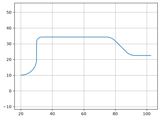
You can also modify our path in the same ways as any other gdsfactory object:
- Manipulation with
move(),rotate(),mirror(), etc - Accessing properties like
xmin,y,center,bbox, etc
P.movey(10)
P.xmin = 20
P.plot()
You can also check the length of the curve with the length() method:
P.length()
105.341
CrossSection
gf.CrossSection is the union of kfactory's DCrossSection and DAsymmetricCrossSection, not a constructor. Build a profile with gf.cross_section.cross_section() or a preset. Auxiliary strips are (layer, minimum, maximum) tuples in micrometers; get_sections() returns the main strip first, then normalized auxiliary strips.
Option 1: Single layer and width
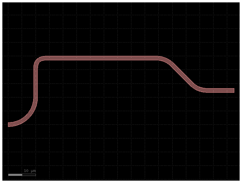
For a single layer, pass a constant width directly to extrude():
# Extrude the Path and the cross-section.
# The extrude function converts a 1D path into a 2D shape by giving it a specified width.

c = gf.path.extrude(P, layer=(1, 0), width=1.5)
c.plot()
Option 2: Arbitrary Cross-section
You can also extrude an arbitrary cross_section.
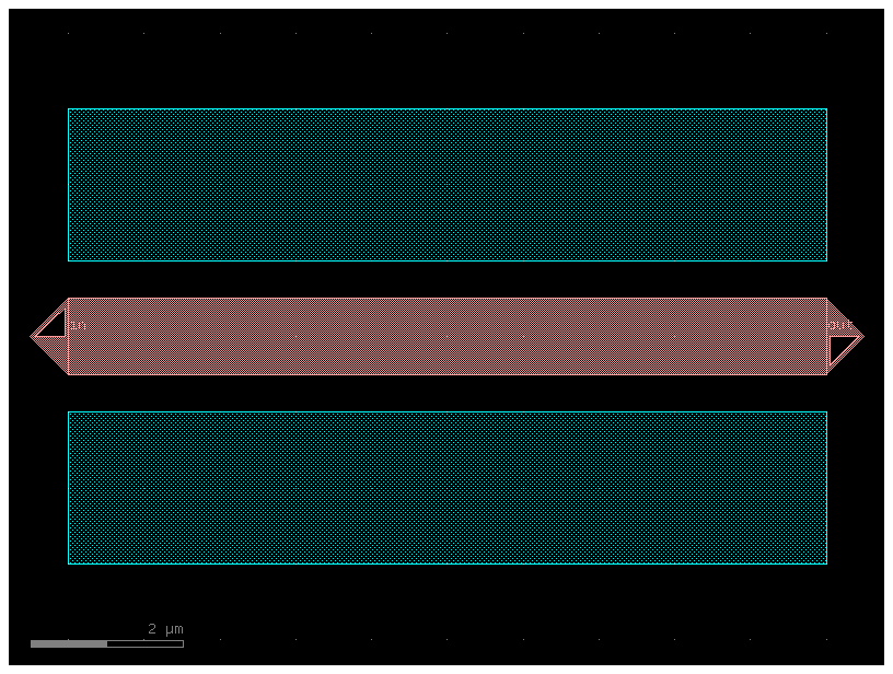
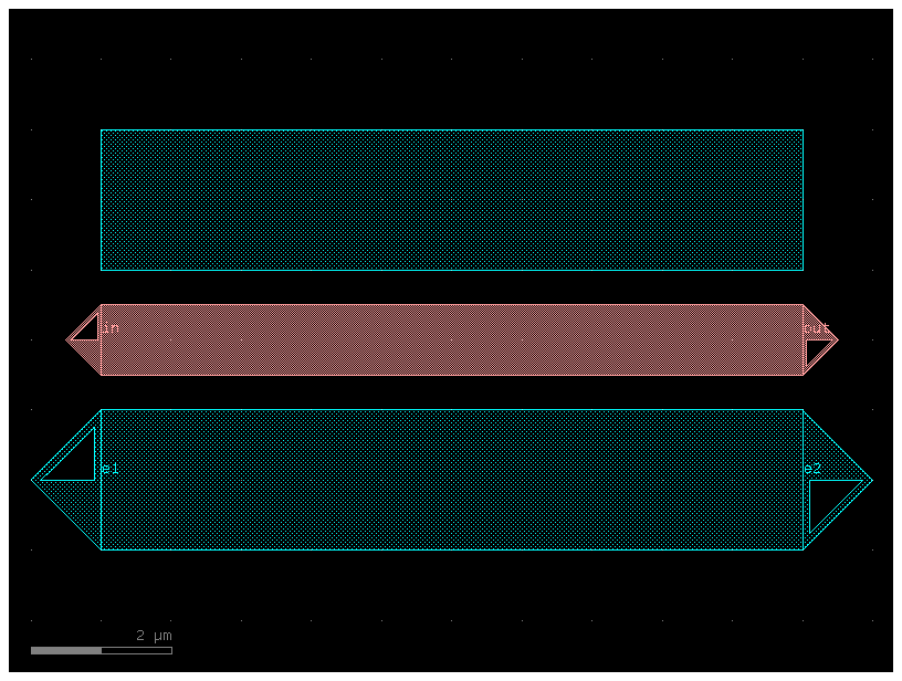
Now, what if we want a more complicated straight? For instance, in some photonic applications it is helpful to have a shallow etch that appears on either side of the straight (often called a trench or sleeve). Additionally, it might be nice to have a port on either end of the center section so we can snap other geometries to it. Let us try adding something like that in:
p = gf.path.straight()

# The code first defines three (layer, minimum, maximum) strips, each representing a part of the total cross-section.
# s0: The central core section. It is 1 µm wide, centered at an offset of 0, and is on layer (1, 0).
# s1: A side section. It is 2 µm wide, its center is offset by +2 µm from the main centerline, and it is on layer (2, 0).
# s2: Another side section, identical to s1 but offset by -2 µm.
s0 = ((1, 0), 0 - 1 / 2, 0 + 1 / 2)
s1 = ((2, 0), 2 - 2 / 2, 2 + 2 / 2)
s2 = ((2, 0), -2 - 2 / 2, -2 + 2 / 2)
x = gf.cross_section.cross_section(width=None, sections=(s0, s1, s2))

c = gf.path.extrude(p, cross_section=x, ports={0: ("in", "out", "optical")})
c.draw_ports()
c.plot()
Select additional ports at extrusion time. Indices refer to get_sections(),
not the input order: normalized auxiliary strips are sorted by layer and bounds.
p = gf.path.straight()

# Add a few "sections" to the cross-section.
s0 = ((1, 0), 0 - 1 / 2, 0 + 1 / 2)
s1 = ((2, 0), 2 - 2 / 2, 2 + 2 / 2)
s2 = ((2, 0), -2 - 2 / 2, -2 + 2 / 2)
x = gf.cross_section.cross_section(width=None, sections=(s0, s1, s2))

c = gf.path.extrude(
    p,
    cross_section=x,
    ports={0: ("in", "out", "optical"), 2: ("e1", "e2", "electrical")},
)
c.draw_ports()
c.plot()
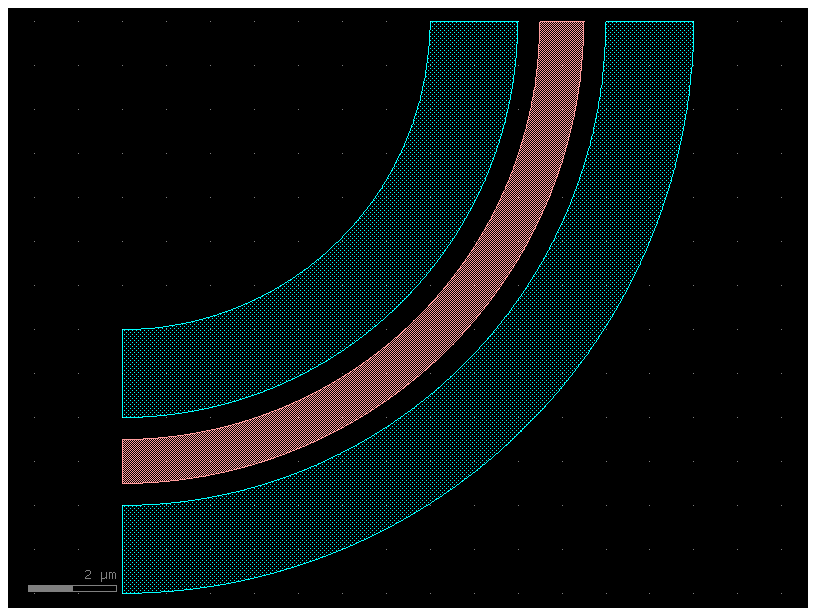
p = gf.path.arc()  # A 1D path in the shape of a 90-degree circular arc is created. This defines the centerline for the extrusion.

# Combine the Path and the cross-section.
b = gf.path.extrude(p, cross_section=x)
b.plot()
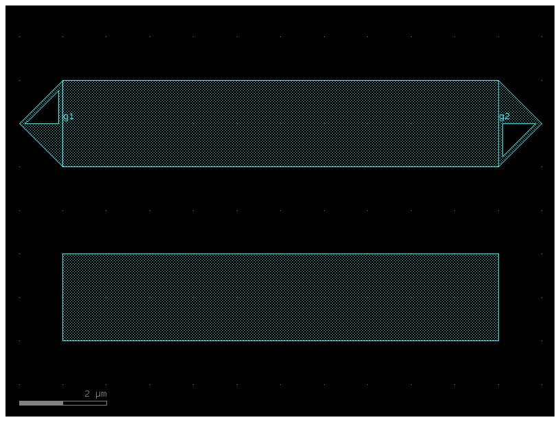
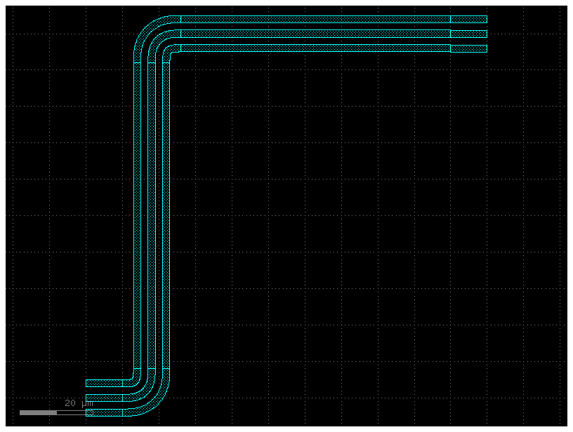
⚠️ Warning! for GS routing. You need to add a centered port for routing to work correctly.
p = gf.path.straight()

# Add GS routing sections.
# GS means ground–signal: two adjacent metal conductors.
s0 = ("M3", 0 - 2 / 2, 0 + 2 / 2)
s1 = ("M3", 4 - 2 / 2, 4 + 2 / 2)
x = gf.cross_section.cross_section(width=None, sections=(s0, s1), radius=8)
c = gf.path.extrude(p, cross_section=x, ports={0: ("g1", "g2", "electrical")})
pad = c
c_copy = c.copy()
c_copy.draw_ports()
c_copy.plot()
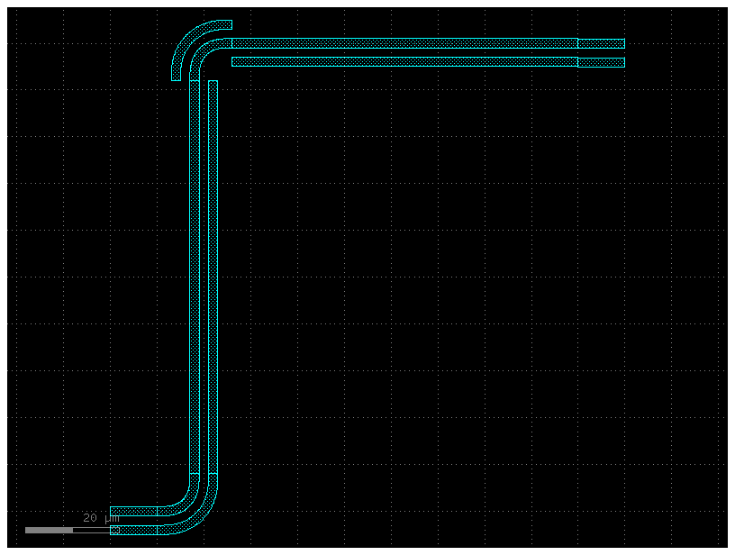
⚠️ Warning! for GS routing. You need to add a centered port for routing to work correctly.
# Do not do this for GS routing. See solution below.
c2 = gf.Component()
pad1 = c2 << pad
pad2 = c2 << pad
pad2.move((100, 100))


# The gf.routing.route_bundle function is a powerful auto-router for creating multiple, parallel waveguide connections.
# [pad1.ports["g2"]]: A list of the starting ports for the routes.
# [pad2.ports["g1"]]: A list of the ending ports for the routes.
# sort_ports=True: An option that helps the router find the optimal, non-crossing paths when routing multiple waveguides.
# bend='bend_euler': Specifies that any curves in the route should be smooth Euler bends.
gf.routing.route_bundle(
    c2,
    [pad1.ports["g2"]],
    [pad2.ports["g1"]],
    cross_section=x,
    sort_ports=True,
    bend="bend_euler",
)
c2.plot()
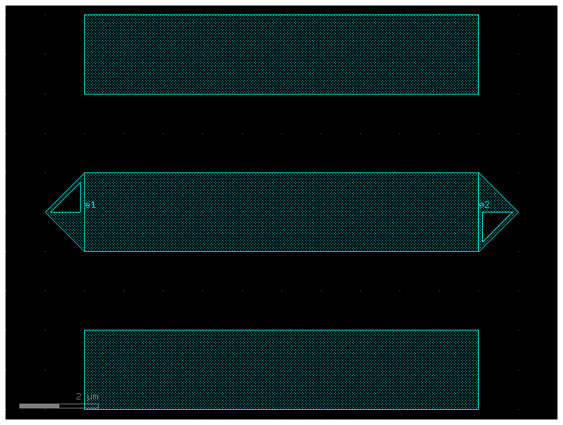
For GSG (ground–signal–ground), the main port is centered on the signal conductor and the two ground conductors are symmetric.
p = gf.path.straight()

# Add a few "sections" to the cross-section
g = ("M3", 0 - 2 / 2, 0 + 2 / 2)
s0 = ("M3", -4 - 2 / 2, -4 + 2 / 2)
s1 = ("M3", 4 - 2 / 2, 4 + 2 / 2)
x = gf.cross_section.cross_section(width=None, sections=(g, s0, s1), radius=8)
c = gf.path.extrude(p, cross_section=x, ports={0: ("e1", "e2", "electrical")})
c_copy = c.copy()
c_copy.draw_ports()
c_copy.plot()
c2 = gf.Component()
pad1 = c2 << c
pad2 = c2 << c
pad2.move((100, 100))
# The bend defaults to wire_corner_sections, which draws every section of the cross-section at the corner.
gf.routing.route_bundle(
    c2, [pad1.ports["e2"]], [pad2.ports["e1"]], cross_section=x, port_type="electrical"
)
c2.plot()
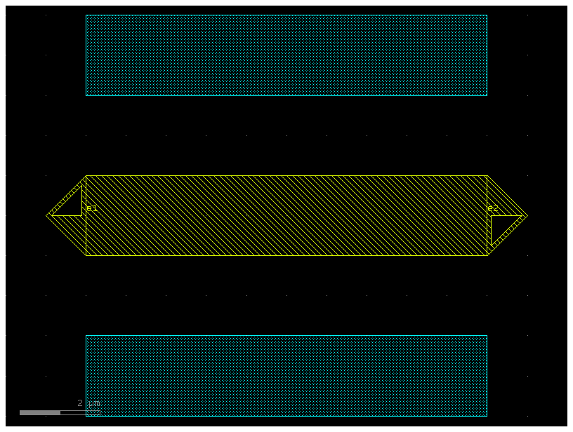
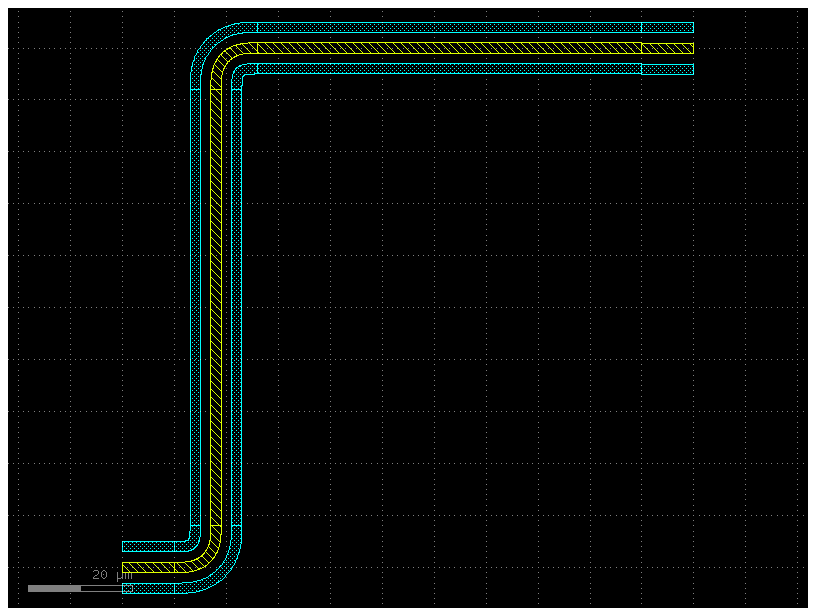
For GS routing the recommended solution is adding a dummy / abstract layer in the middle, where we add the ports.
p = gf.path.straight()

# Add GS routing sections.
# 99, 0 is an abstract layer that can be used to add ports to the path.
s0 = ((99, 0), 0 - 2 / 2, 0 + 2 / 2)
s1 = ((2, 0), -4 - 2 / 2, -4 + 2 / 2)
s2 = ((2, 0), +4 - 2 / 2, +4 + 2 / 2)
x = gf.cross_section.cross_section(width=None, sections=(s0, s1, s2), radius=8)
c = gf.path.extrude(p, cross_section=x, ports={0: ("e1", "e2", "electrical")})
pad = c
c_copy = c.copy()
c_copy.draw_ports()
c_copy.plot()
c2 = gf.Component()
pad1 = c2 << c
pad2 = c2 << c
pad2.move((100, 100))
gf.routing.route_bundle(
    c2,
    [pad1.ports["e2"]],
    [pad2.ports["e1"]],
    cross_section=x,
    port_type="optical",
    bend="bend_euler",
    raise_on_error=True,
)
c2.plot()
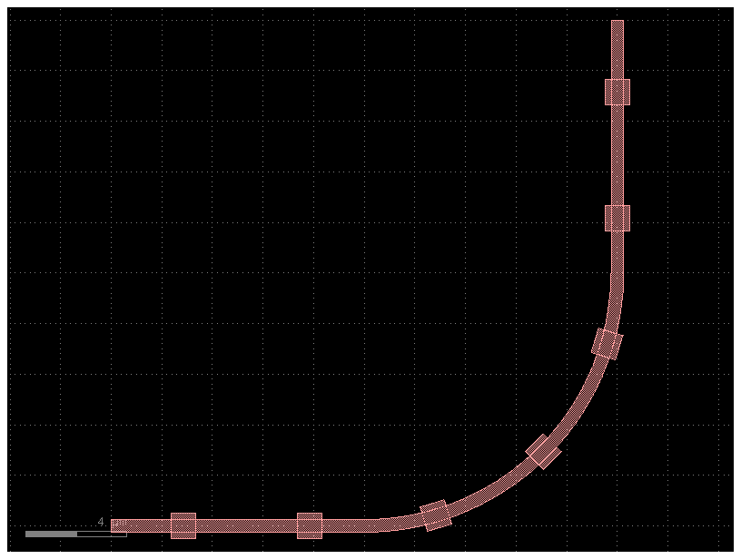
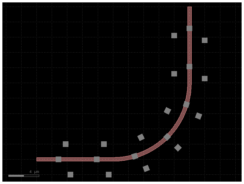
Option 3: Components along a path
You can also place components along a path, which is useful for wiring vias. A via is a vertical electrical connection that goes through the insulating layers of an integrated circuit to connect different layers of horizontal metal wiring.
# Components along a path are placed explicitly, not stored in a profile.
p = gf.path.straight() + gf.path.arc(10) + gf.path.straight()
x = gf.cross_section.strip()
c = p.extrude(x)
c << gf.path.along_path(
    p, component=gf.c.rectangle(size=(1, 1), centered=True), spacing=5, padding=2
)
c.plot()
p = gf.path.straight() + gf.path.arc(10) + gf.path.straight()
c = p.extrude("strip")
for offset in (0, 2, -2):
    c << gf.path.along_path(
        p.copy().offset(offset), component=gf.c.via1(), spacing=5, padding=2
    )
c.plot()
Path
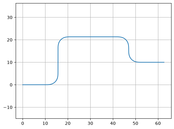
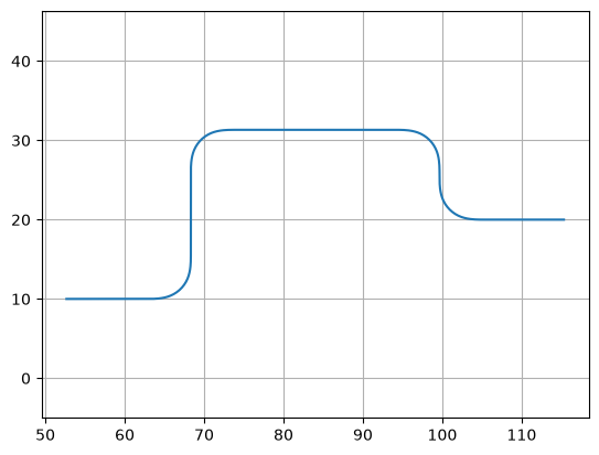
You can pass append() lists of path segments. This makes it easy to combine paths very quickly.
Below we show 3 examples using this functionality:
Example 1: Assemble a complex path by making a list of paths and passing it to append().
import gdsfactory as gf

P = gf.Path()

# Create the basic Path components.
left_turn = gf.path.euler(radius=4, angle=90)
right_turn = gf.path.euler(radius=4, angle=-90)
straight = gf.path.straight(length=10)

# Assemble a complex path by making a list of paths and passing it to `append()`.
# .append([...]): This method takes a list of path factories and adds them sequentially to the end of the existing path P.
# Each new segment starts where the previous one ended, creating a single, continuous path.
P.append(
    [
        straight,
        left_turn,
        straight,
        right_turn,
        straight,
        straight,
        right_turn,
        left_turn,
        straight,
    ]
)

P.plot()
P = (
    straight
    + left_turn
    + straight
    + right_turn
    + straight
    + straight
    + right_turn
    + left_turn
    + straight
)
P.plot()
Example 2: Create an "S-turn" just by making a list of [left_turn,
right_turn].
P = gf.Path()

# Create an "S-turn" by making a list.
s_turn = [left_turn, right_turn]

P.append(s_turn)
P.plot()
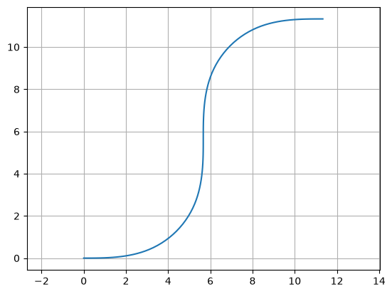
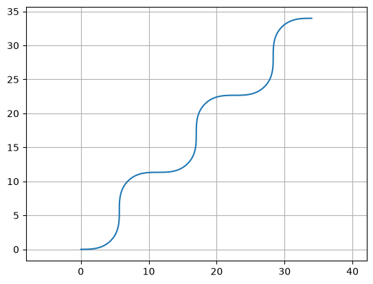
Example 3: Repeat the S-turn 3 times by nesting our S-turn list in another list. Nesting means placing one data structure inside another of the same type. In this context, it means creating a "list of lists."
P = gf.Path()

# Create an "S-turn" using a list.
s_turn = [left_turn, right_turn]

# Repeat the S-turn 3 times by nesting our S-turn list 3x times in another list.
triple_s_turn = [s_turn, s_turn, s_turn]

P.append(triple_s_turn)
P.plot()
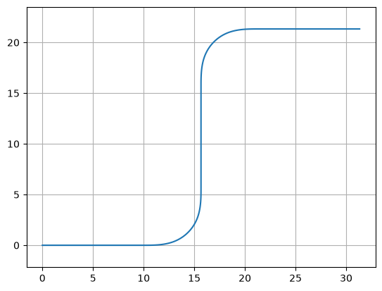
Note you can also use the Path() constructor to immediately construct your Path:
P = gf.Path([straight, left_turn, straight, right_turn, straight])
P.plot()
Waypoint smooth paths
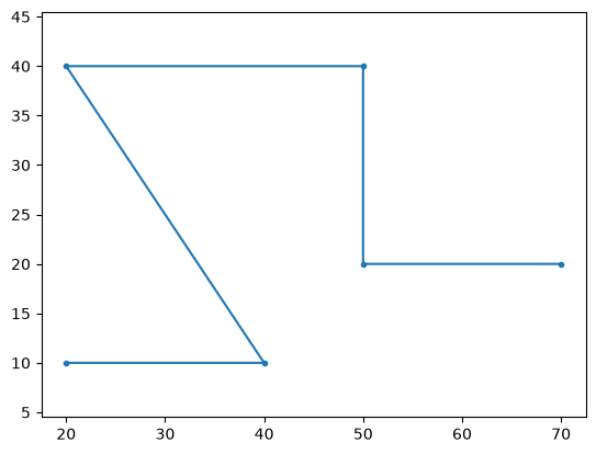
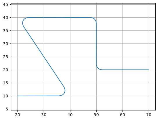
You can also build smooth paths between waypoints with the smooth() function.
points = np.array([(20, 10), (40, 10), (20, 40), (50, 40), (50, 20), (70, 20)])
plt.plot(points[:, 0], points[:, 1], ".-")

# This functionensures that one unit on the x-axis is the same length as one unit on the y-axis.
# This is crucial for plots where the geometric shape is important.
plt.axis("equal")
(np.float64(17.5), np.float64(72.5), np.float64(8.5), np.float64(41.5))
points = np.array([(20, 10), (40, 10), (20, 40), (50, 40), (50, 20), (70, 20)])

P = gf.path.smooth(
    points=points,
    radius=2,
    bend=gf.path.euler,  # Alternatively, use pp.arc, which will create a constant-radius bend.
    use_eff=False,
)
P.plot()
Waypoint sharp paths
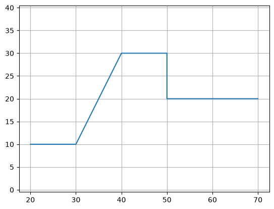
It is also possible to make more traditional angular paths (e.g. electrical wires) in a few different ways.
Example 1: Using a simple list of points:
P = gf.Path([(20, 10), (30, 10), (40, 30), (50, 30), (50, 20), (70, 20)])
P.plot()
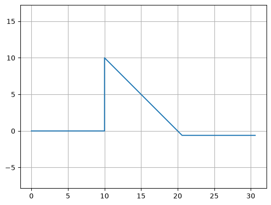
Example 2: Using the "turn and move" method, where you manipulate the end angle of the path so that when you append points to it they are in the correct direction. Note: It is crucial that the number of points per straight section is set to 2 (gf.path.straight(length, num_pts = 2)) otherwise the extrusion algorithm will show defects.
P = gf.Path()
P += gf.path.straight(length=10, npoints=2)
P.end_angle += 90  # "Turn" 90 deg (left).
P += gf.path.straight(length=10, npoints=2)  # "Walk" length of 10.
P.end_angle += -135  # "Turn" -135 degrees (right).
P += gf.path.straight(length=15, npoints=2)  # "Walk" length of 15.
P.end_angle = 0  # Force the direction to be 0 degrees.
P += gf.path.straight(length=10, npoints=2)
P.plot()
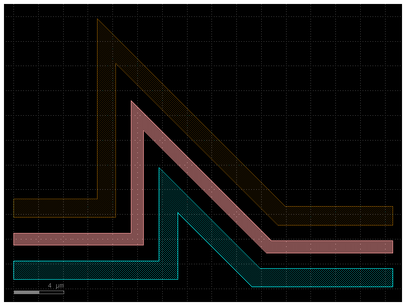
s0 = ((1, 0), 0 - 1 / 2, 0 + 1 / 2)
s1 = ((2, 0), 2.5 - 1.5 / 2, 2.5 + 1.5 / 2)
s2 = ((3, 0), -2.5 - 1.5 / 2, -2.5 + 1.5 / 2)
X = gf.cross_section.cross_section(width=None, sections=[s0, s1, s2])
c = gf.path.extrude(P, X)
c.plot()
Custom curves
Now let us have some fun and try to make a loop-de-loop structure with parallel straights and several ports.
To create a new type of curve we simply make a function that produces an array
of points. The best way to do that is to create a function which allows you to
specify a large number of points along that curve -- in the case shown below, the
looploop() function outputs 1000 points along a looping path. Later, if we
want to reduce the number of points in our geometry we can easily simplify the
path.
def looploop(num_pts=1000):
    """Simple limacon looping curve."""

    # This line creates an array of num_pts evenly spaced numbers ranging from -π to 0. This array represents the angle t in polar coordinates.
    t = np.linspace(-np.pi, 0, num_pts)
    r = (
        20 + 25 * np.sin(t)
    )  # This line calculates the radius r for each corresponding angle t using the polar equation for a limaçon curve.

    # # These lines convert the polar coordinates (r, t) into standard Cartesian coordinates (x, y), which are needed for plotting.
    x = r * np.cos(t)
    y = r * np.sin(t)

    # The separate x and y arrays are combined into a single NumPy array of coordinate pairs, which is then returned by the function.
    return np.array((x, y)).T


# Create the path points.
P = gf.Path()
P.append(gf.path.arc(radius=10, angle=90))
P.append(gf.path.straight())
P.append(gf.path.arc(radius=5, angle=-90))
P.append(looploop(num_pts=1000))
P.rotate(-45)

# Create the cross-section.
s0 = ((1, 0), 0 - 1 / 2, 0 + 1 / 2)
s1 = ((2, 0), 2 - 0.5 / 2, 2 + 0.5 / 2)
s2 = ((3, 0), 4 - 0.5 / 2, 4 + 0.5 / 2)
s3 = ((4, 0), 0 - 1 / 2, 0 + 1 / 2)
X = gf.cross_section.cross_section(width=None, sections=(s0, s1, s2, s3))

c = gf.path.extrude(P, X)
c.plot()
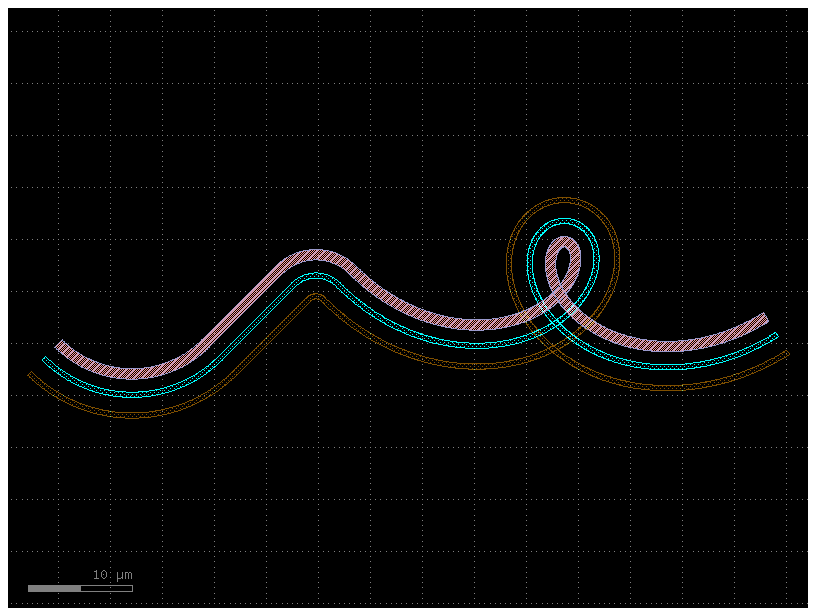
You can create Paths from any array of points -- just be sure that they form
smooth curves! If we examine our path P we can see that we have effortlessly
created a long list of points:
path_points = P.points  # Curve points are stored as a numpy array in P.points.
print(np.shape(path_points))  # The shape of the array is Nx2.
print(len(P))  # Equivalently, use len(P) to see how many points are inside.
(1092, 2)
1092
Simplifying / reducing point usage
One of the primary concerns of generating smooth curves is that too many points
are generated, inflating file sizes and making boolean operations
computationally expensive. Fortunately, PHIDL has a fast implementation of the
Ramer-Douglas–Peucker
algorithm
that lets you reduce the number of points in a curve without changing its shape.
All that needs to be done when you make a component() is extruding the path with a cross_section, you need to specify the
simplify argument.
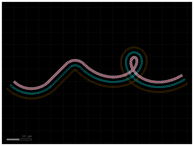
If we specify simplify = 1e-3, the number of points in the line drops from
12,000 to 4,000, and the remaining points form a line that is identical to
within 1e-3 distance from the original (for the default 1 micron unit size,
this corresponds to 1 nanometer resolution):
# The remaining points form a identical line to within `1e-3` from the original.
c = gf.path.extrude(p=P, cross_section=X, simplify=1e-3)
c.plot()
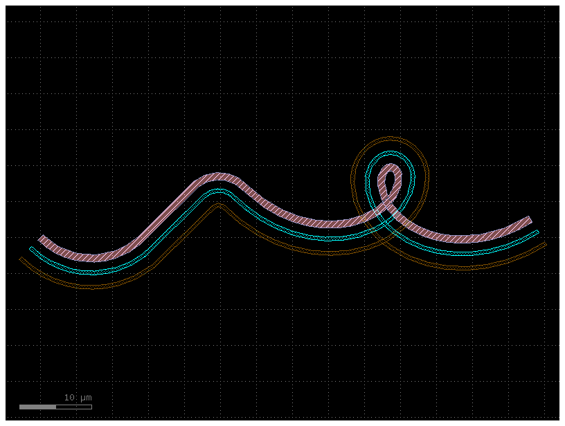
Let us say we need fewer points. We can increase the simplify tolerance by specifying simplify = 1e-1. This drops the number of points to ~400 points and they form a line that is identical to within 1e-1 distance from the original:
c = gf.path.extrude(P, cross_section=X, simplify=1e-1)
c.plot()
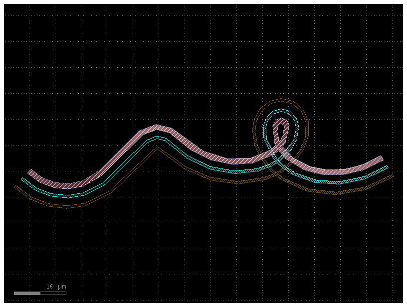
Taken to absurdity, what happens if we set simplify = 0.3? Once again, the
~200 remaining points form a line that is within 0.3 units from the original
-- but that line will look pretty bad.
c = gf.path.extrude(P, cross_section=X, simplify=0.3)
c.plot()
Curvature calculation
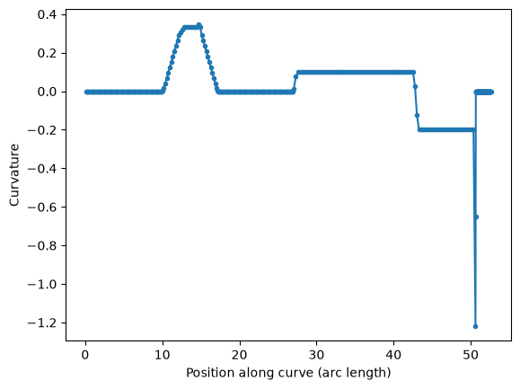
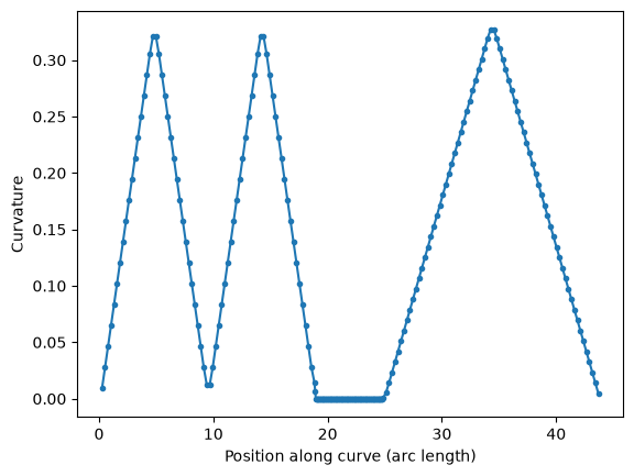
The Path class has a curvature() method that computes the curvature K of
your smooth path (K = 1/(radius of curvature)). This can be helpful for
verifying that your curves transition smoothly such as in track-transition
curves (also known as
"Euler" bends in the photonics world). Euler bends have lower mode-mismatch loss as explained in this paper
Note this curvature is numerically computed, so areas in which the curvature jumps instantaneously (such as between an arc and a straight segment) will be slightly interpolated, and sudden changes in point density along the curve can cause discontinuities.
straight_points = 100

P = gf.Path()
P.append(
    [
        gf.path.straight(
            length=10, npoints=straight_points
        ),  # Should have a curvature of 0
        gf.path.euler(
            radius=3, angle=90, p=0.5, use_eff=False
        ),  # Euler straight-to-bend transition with min. bend radius of 3 (max curvature of 1/3)
        gf.path.straight(
            length=10, npoints=straight_points
        ),  # Should have a curvature of 0
        gf.path.arc(radius=10, angle=90),  # Should have a curvature of 1/10
        gf.path.arc(radius=5, angle=-90),  # Should have a curvature of -1/5
        gf.path.straight(
            length=2, npoints=straight_points
        ),  # Should have a curvature of 0
    ]
)

P.plot()
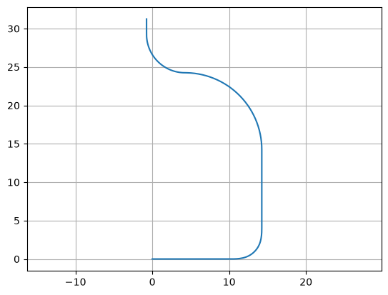
Arc paths are equivalent to bend_circular and euler paths are equivalent to bend_euler.
# The .curvature() method of the Path object P is called.
# It returns two arrays: s, which contains the cumulative distance (arc length) at each point along the path,
# and K, which contains the corresponding curvature at that point. (Curvature is the reciprocal of the bend radius).
s, K = P.curvature()

# This plots the arc length s on the x-axis and the curvature K on the y-axis.
# The ".-" format string specifies that the plot should be a line with a dot marker at each data point.
plt.plot(s, K, ".-")
plt.xlabel("Position along curve (arc length)")
plt.ylabel("Curvature")
Text(0, 0.5, 'Curvature')
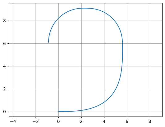
P = gf.path.euler(radius=3, angle=90, p=1.0, use_eff=False)
P.append(gf.path.euler(radius=3, angle=90, p=0.2, use_eff=False))
P.append(gf.path.euler(radius=3, angle=90, p=0.0, use_eff=False))
P.plot()
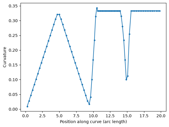
s, K = P.curvature()
plt.plot(s, K, ".-")
plt.xlabel("Position along curve (arc length)")
plt.ylabel("Curvature")
Text(0, 0.5, 'Curvature')
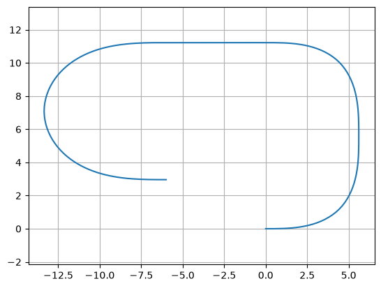
You can compare two 90 degrees euler bends with 180 euler bend.
A 180 euler bend is shorter, and has less loss than two 90 degrees euler bend.
straight_points = 100

P = gf.Path()
P.append(
    [
        gf.path.euler(radius=3, angle=90, p=1, use_eff=False),
        gf.path.euler(radius=3, angle=90, p=1, use_eff=False),
        gf.path.straight(length=6, npoints=100),
        gf.path.euler(radius=3, angle=180, p=1, use_eff=False),
    ]
)

P.plot()
s, K = P.curvature()
plt.plot(s, K, ".-")
plt.xlabel("Position along curve (arc length)")
plt.ylabel("Curvature")
Text(0, 0.5, 'Curvature')
Transitioning between cross-sections
gf.path.transition() pairs two profiles in an extrusion-time Transition. extrude_transition() matches their main strips and then auxiliary strips by layer and signed-bound order. Use section_pairs for explicit index pairs. Section names are not part of a profile.
# Create our first Cross-section.
import gdsfactory as gf

s0 = ((2, 0), 0 - 1.2 / 2, 0 + 1.2 / 2)
s1 = ((3, 0), 0 - 2.2 / 2, 0 + 2.2 / 2)
s2 = ((1, 0), 3 - 1.1 / 2, 3 + 1.1 / 2)
X1 = gf.cross_section.cross_section(width=None, sections=[s0, s1, s2])

# Create the second Cross-section that we want to transition to.
s0 = ((2, 0), 0 - 1 / 2, 0 + 1 / 2)
s1 = ((3, 0), 0 - 3.5 / 2, 0 + 3.5 / 2)
s2 = ((1, 0), 5 - 3 / 2, 5 + 3 / 2)
X2 = gf.cross_section.cross_section(width=None, sections=[s0, s1, s2])

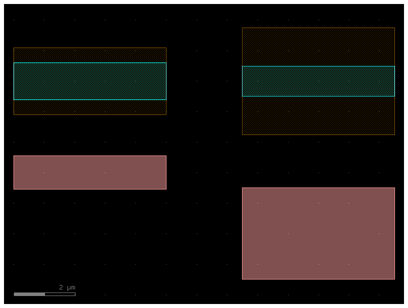
# To show the cross-sections, let us now create two paths and create components by extruding them.
P1 = gf.path.straight(length=5)
P2 = gf.path.straight(length=5)
wg1 = gf.path.extrude(P1, X1)
wg2 = gf.path.extrude(P2, X2)

# Place both cross-section components and quickplot them,
# Quickplot is designed to create a wide variety of complex graphs with a simple, concise syntax, making it ideal for quick data exploration.
c = gf.Component()
wg1ref = c << wg1
wg2ref = c << wg2
wg2ref.movex(7.5)

c.plot()
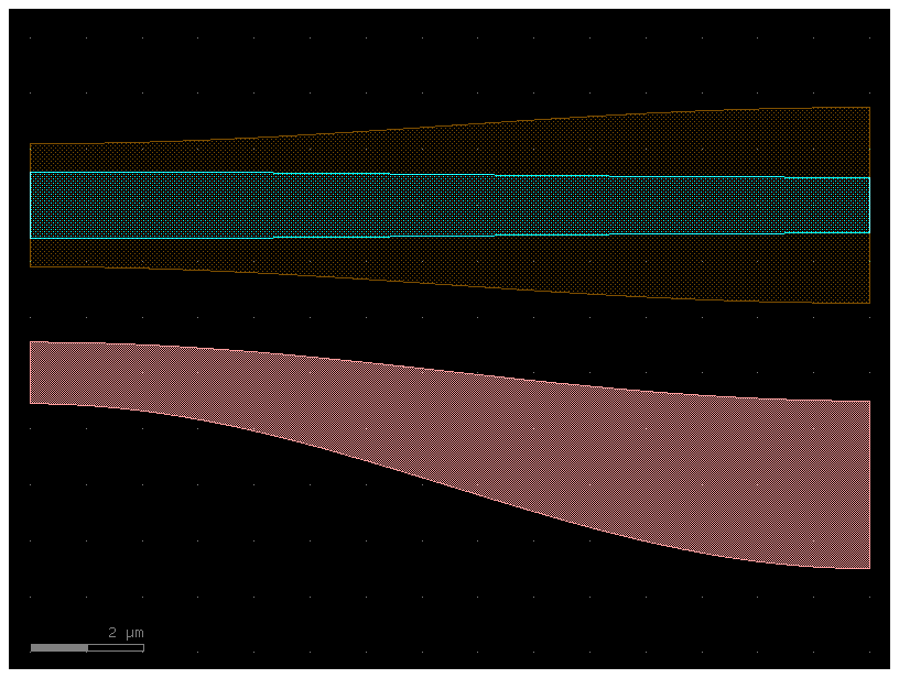
Now we can create the transitional cross-section by calling a transition() with
these two cross-sections as the input. If we want the width to vary as a smooth
sinusoid between the sections, we can set width_type to 'sine'
(alternatively we could also use 'linear').
# Create the transitional cross-section.
Xtrans = gf.path.transition(cross_section1=X1, cross_section2=X2, width_type="sine")

# Create a Path for the transitional cross-section to follow.
P3 = gf.path.straight(length=15, npoints=100)

# Use the transitional cross-section to create a component.
straight_transition = gf.path.extrude_transition(P3, Xtrans)
straight_transition.plot()
Now that we have all of our components, let us proceed to connect() everything and see
what it looks like:
c = gf.Component("transition_demo")

wg1ref = c << wg1
wgtref = c << straight_transition
wg2ref = c << wg2

wgtref.connect("o1", wg1ref.ports["o2"], mirror=True)
wg2ref.connect("o1", wgtref.ports["o2"], mirror=True)

c.plot()
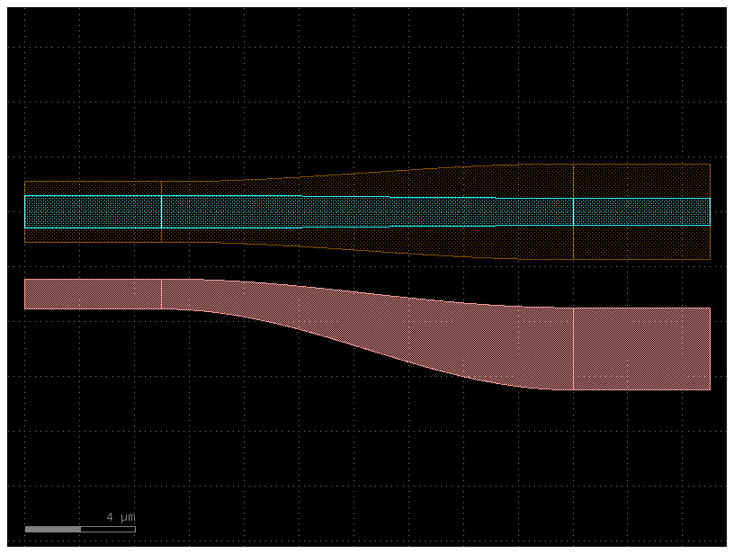
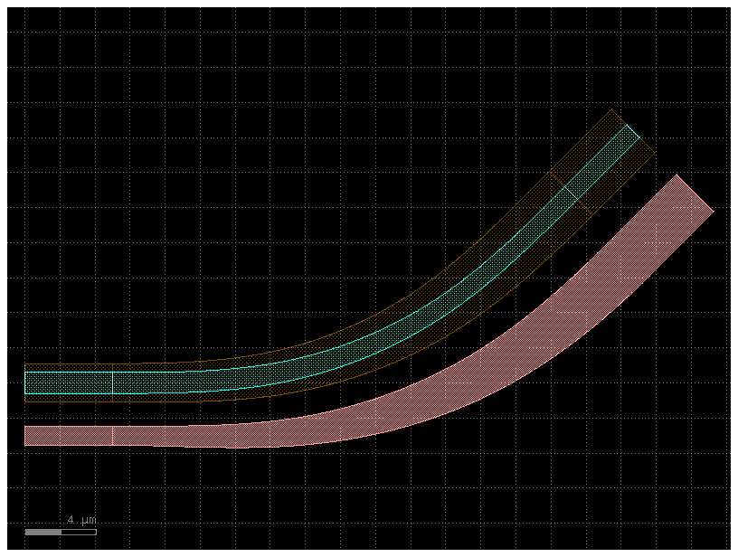
Note that since transition() outputs a Transition, we can make the transition follow an arbitrary path:
# Transition along a curving path.
P4 = gf.path.euler(radius=25, angle=45, p=0.5, use_eff=False)
wg_trans = gf.path.extrude_transition(P4, Xtrans)

c = gf.Component("demo_transition")
wg1_ref = c << wg1  # First cross-section component.
wg2_ref = c << wg2
wgt_ref = c << wg_trans

wgt_ref.connect("o1", wg1_ref.ports["o2"], mirror=True)
wg2_ref.connect("o1", wgt_ref.ports["o2"], mirror=True)

c.plot()
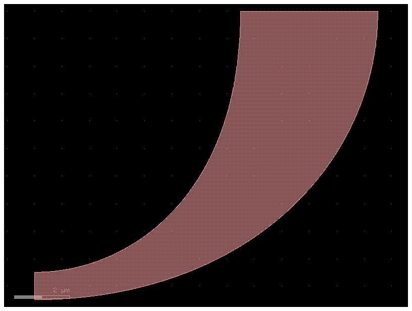
You can also extrude an arbitrary transition:
w1 = 1
w2 = 5
x1 = gf.get_cross_section("strip", width=w1)
x2 = gf.get_cross_section("strip", width=w2)
transition = gf.path.transition(x1, x2)
p = gf.path.arc(radius=10)
c = gf.path.extrude_transition(p, transition)
c.plot()
Asymmetric transition
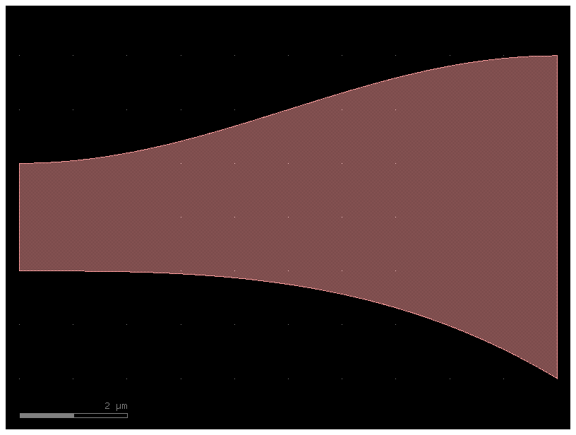
In some cases, you may want the edges of the transition to follow a different function.
This can be done by using the transition_asymmetric() function.
In this case, the argument width_type of transition is split into width_type1, corresponding to the lower edge, and width_type2, corresponding to the upper edge of the transition.
As in the case of transition(), the user can define their own transition function.
Let us look at an example where the upper edge follows the sinusoidal (default) transition of the width, while the lower follows a user-defined polynomial.
import gdsfactory as gf


# Define a custom polynomial transition function from y1 -> y2, for t ∈ [0,1].
def polynomial(t: float, y1: float, y2: float) -> float:
    return (y2 - y1) * t**3 + y1


w1 = 2
w2 = 6
length = 10
cs1 = gf.get_cross_section("strip", width=w1)
cs2 = gf.get_cross_section("strip", width=w2)

transition = gf.path.transition_asymmetric(
    cs1, cs2, width_type1=polynomial, width_type2="sine"
)
p = gf.path.straight(length, npoints=100)
c = gf.path.extrude_transition(p, transition)

c.plot()
Variable width / offset
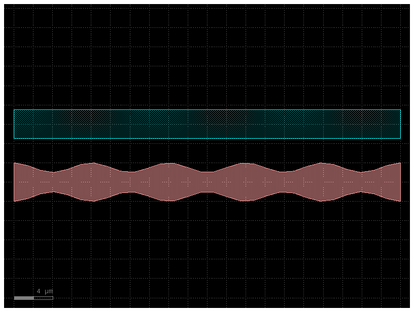
Pass vectorized width_function or offset_function to extrude(). A single function applies to the main strip; a dictionary selects indices from get_sections(). The parameter runs from 0 at the start to 1 at the end. The static profile is unchanged.
import numpy as np

import gdsfactory as gf


def my_custom_width_fun(t):
    # Note: Custom width/offset functions MUST be vectorizable --
    # you must be able to call them with an array input like my_custom_width_fun([0, 0.1, 0.2, 0.3, 0.4]).
    num_periods = 5

    # np.cos(...): This is the core cosine function from the NumPy library, which generates a wave that oscillates between -1 and 1.
    # 2 * np.pi * t * num_periods: This part calculates the angle (in radians) for the cosine function.
    # It determines the frequency of the wave, i.e., how many full cycles (num_periods) it completes over a given time t.
    # This adds a vertical offset of 3 to the wave. Instead of oscillating between -1 and 1, the wave now oscillates between 2 (3 - 1) and 4 (3 + 1).
    return 3 + np.cos(2 * np.pi * t * num_periods)


P = gf.path.straight(length=40, npoints=30)

# Create two cross-sections: one fixed width, one modulated by my_custom_offset_fun.
s0 = ((2, 0), -6 - 3 / 2, -6 + 3 / 2)
s1 = ((1, 0), 0 - 4.0 / 2, 0 + 4.0 / 2)
X = gf.cross_section.cross_section(width=None, sections=(s0, s1))

# # Extrude the path to create the component.
c = gf.path.extrude(P, cross_section=X, width_function={1: my_custom_width_fun})
c.plot()
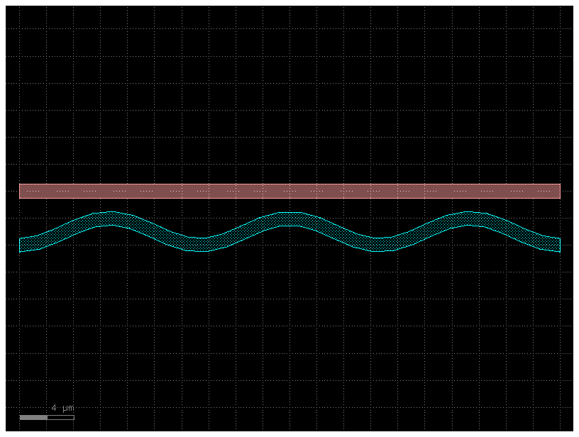
We can do the same thing with the offset argument:
def my_custom_offset_fun(t):
    num_periods = 3
    return 3 + np.cos(2 * np.pi * t * num_periods)


P = gf.path.straight(length=40, npoints=30)

s0 = ((1, 0), 0 - 1 / 2, 0 + 1 / 2)
s1 = ((2, 0), 0 - 1 / 2, 0 + 1 / 2)
X = gf.cross_section.cross_section(width=None, sections=(s0, s1))

c = gf.path.extrude(
    P,
    cross_section=X,
    offset_function={1: my_custom_offset_fun},
    ports={1: ("clad1", "clad2", "optical")},
)
c.plot()
Offsetting a Path
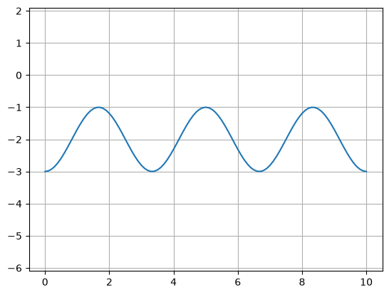
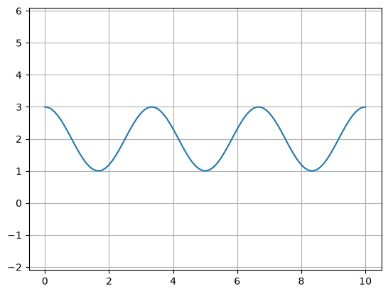
Sometimes it is convenient to start with a simple path and offset the line it
follows to suit your needs (without using a custom-offset cross-section). Here,
we start with two copies of a simple straight path and use the offset()
function to directly modify each path.
def my_custom_offset_fun(t):
    num_periods = 3
    return 2 + np.cos(2 * np.pi * t * num_periods)


P1 = gf.path.straight(npoints=101)
P1.offset(offset=my_custom_offset_fun)
P1.plot()
P2 = P1.copy()  # Make a copy of the path.
P2.mirror((1, 0))  # Mirror across X-axis.
P2.plot()
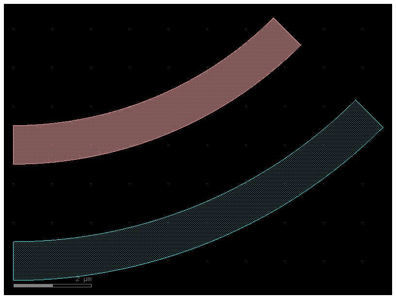
P = gf.path.arc(radius=10, angle=45)

s0 = ((2, 0), 3 - 1 / 2, 3 + 1 / 2)
s1 = ((1, 0), 0 - 1 / 2, 0 + 1 / 2)
X = gf.cross_section.cross_section(width=None, sections=(s0, s1))
c = gf.path.extrude(P, X, ports={1: ("o1", "o2", "optical")})
c.plot()
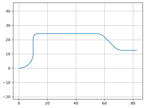
P = gf.Path()
P.append(gf.path.arc(radius=10, angle=90))  # Circular arc.
P.append(gf.path.straight(length=10))  # Straight section.
P.append(gf.path.euler(radius=3, angle=-90))  # Euler bend (aka "racetrack" curve).
P.append(gf.path.straight(length=40))
P.append(gf.path.arc(radius=8, angle=-45))
P.append(gf.path.straight(length=10))
P.append(gf.path.arc(radius=8, angle=45))
P.append(gf.path.straight(length=10))

P.plot()
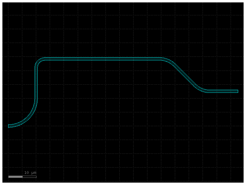
c = gf.path.extrude(P, width=1, layer=(2, 0))
c.plot()
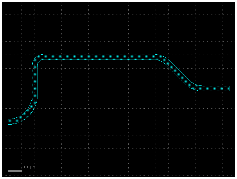
s0 = ((2, 0), 0 - 2 / 2, 0 + 2 / 2)
xs = gf.cross_section.cross_section(width=None, sections=(s0,))
c = gf.path.extrude(P, xs)
c.plot()
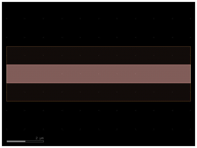
p = gf.path.straight(length=10, npoints=101)
s0 = ((1, 0), 0 - 1 / 2, 0 + 1 / 2)
s1 = ((3, 0), 0 - 3 / 2, 0 + 3 / 2)
x1 = gf.cross_section.cross_section(width=None, sections=(s0, s1))
c = gf.path.extrude(p, x1)
c.plot()
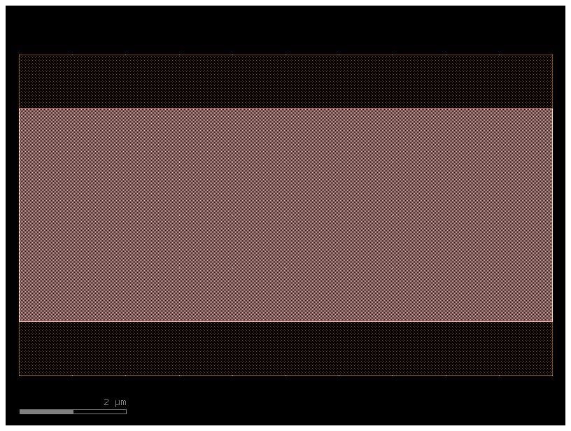
s0 = ((1, 0), 0 - (1 + 3) / 2, 0 + (1 + 3) / 2)
s1 = ((3, 0), 0 - (3 + 3) / 2, 0 + (3 + 3) / 2)
x2 = gf.cross_section.cross_section(width=None, sections=(s0, s1))
c2 = gf.path.extrude(p, x2)
c2.plot()
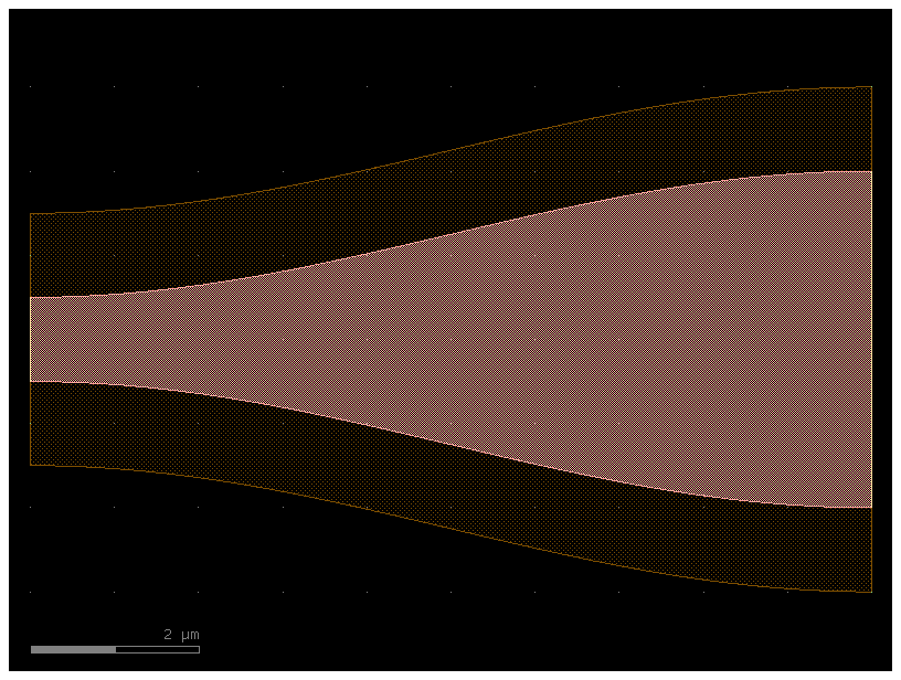
t = gf.path.transition(x1, x2)
c3 = gf.path.extrude_transition(p, t)
c3.plot()
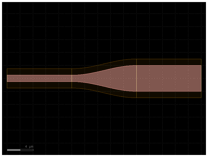
c4 = gf.Component()
start_ref = c4 << c
trans_ref = c4 << c3
end_ref = c4 << c2

trans_ref.connect("o1", start_ref.ports["o2"])
end_ref.connect("o1", trans_ref.ports["o2"])
c4.plot()
Avoiding transitions for specific layers
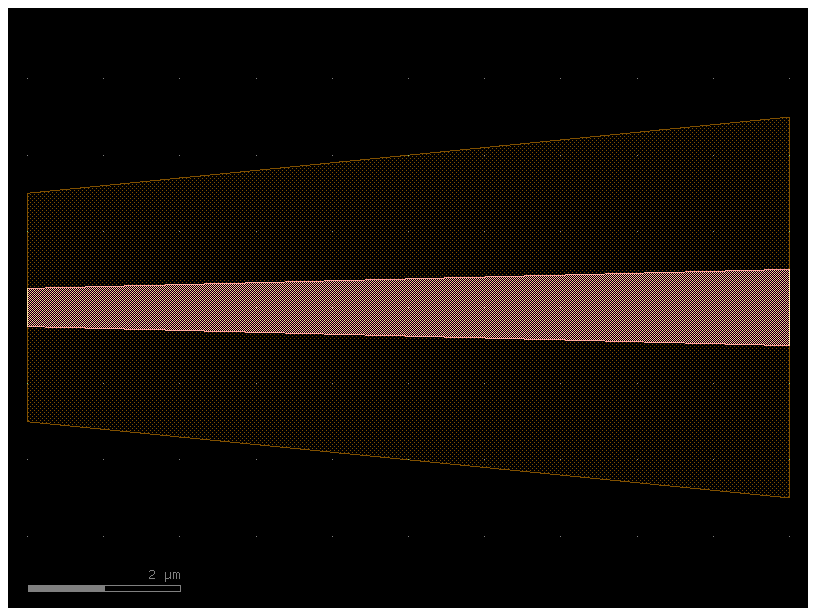
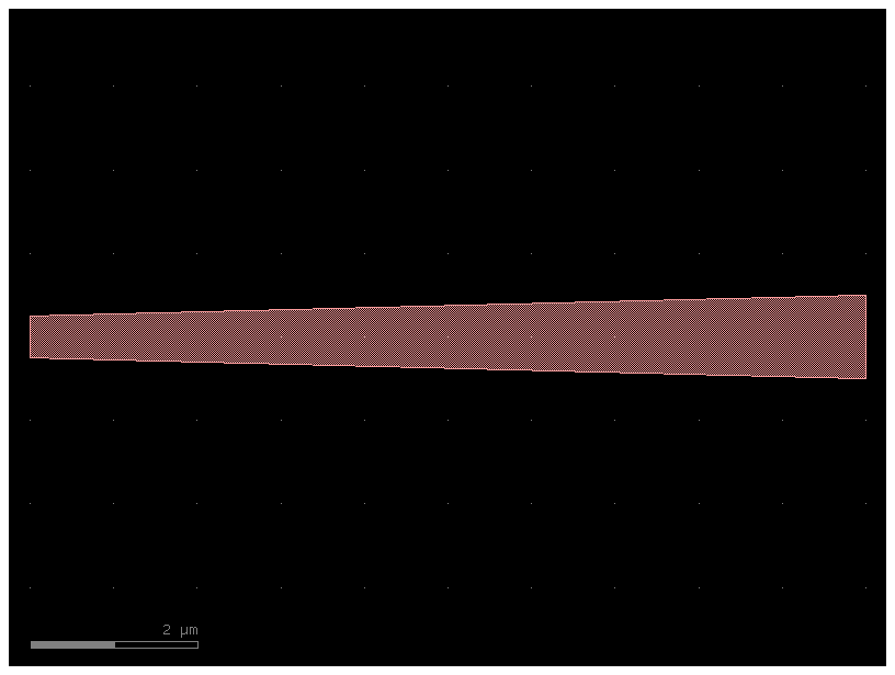
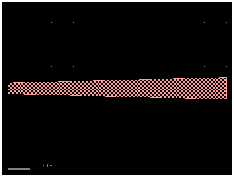
Pairing is by layer, not by section name. Use section_pairs to select pairs explicitly, or skip_transition to omit source-section indices.
import gdsfactory as gf

p = gf.path.straight(length=10, npoints=101)

# Cross-section 1: core + slab on separate layers
s0 = ((1, 0), 0 - 0.5 / 2, 0 + 0.5 / 2)
s1 = ((3, 0), 0 - 3 / 2, 0 + 3 / 2)
x1 = gf.cross_section.cross_section(width=None, sections=(s0, s1))

# Cross-section 2: wider core + wider slab
s0 = ((1, 0), 0 - 1.0 / 2, 0 + 1.0 / 2)
s1 = ((3, 0), 0 - 5 / 2, 0 + 5 / 2)
x2 = gf.cross_section.cross_section(width=None, sections=(s0, s1))

# Both the main core and the auxiliary slab are transitioned.
t_both = gf.path.transition(x1, x2, width_type="linear")
c_both = gf.path.extrude_transition(p, t_both)
c_both.plot()
# Pair only the two main strips. Auxiliary slabs are omitted.
t_core_only = gf.path.transition(x1, x2, width_type="linear")
c_core_only = gf.path.extrude_transition(p, t_core_only, section_pairs=[(0, 0)])
c_core_only.plot()
# The equivalent section-index exclusion is an extrusion option.
t_skip = gf.path.transition(x1, x2, width_type="linear")
c_skip = gf.path.extrude_transition(p, t_skip, skip_transition=[1])
c_skip.plot()
Creating new cross_sections
You can create cross sections in three ways:
- Customize an existing cross-section for example
gf.cross_section.strip. - Define a function that returns a cross_section.
- Construct a kfactory cross-section object directly.
What parameters do cross_section take?
help(gf.cross_section.cross_section)
Help on function cross_section in module gdsfactory.cross_section.utils:

cross_section(width: 'float | None' = 0.5, offset: 'float' = 0, layer: 'typings.LayerSpec | kf.kdb.LayerInfo' = 'WG', sections: 'Sections | None' = None, bbox_layers: 'Sequence[typings.LayerSpec | kf.kdb.LayerInfo] | None' = None, bbox_offsets: 'typings.Floats | None' = None, cladding_layers: 'typings.LayerSpecs | None' = None, cladding_offsets: 'float | typings.Floats | None' = None, cladding_centers: 'float | typings.Floats | None' = None, radius: 'float | None' = None, radius_min: 'float | None' = None, name: 'str | None' = None, kcl: 'kf.KCLayout | None' = None) -> 'CrossSection'
    Build a profile, rounding each signed strip edge with KLayout's DBU rule.

    Auxiliary sections are ``(layer, minimum, maximum)`` tuples in micrometers,
    or kfactory DCrossSectionLayer objects. The main strip stays separate from
    overlapping auxiliary strips. Mirrored auxiliary bands become edge-relative
    enclosures when the main strip is centered; other profiles are asymmetric.
    Port names, dynamic widths and other extrusion options belong to extrude().
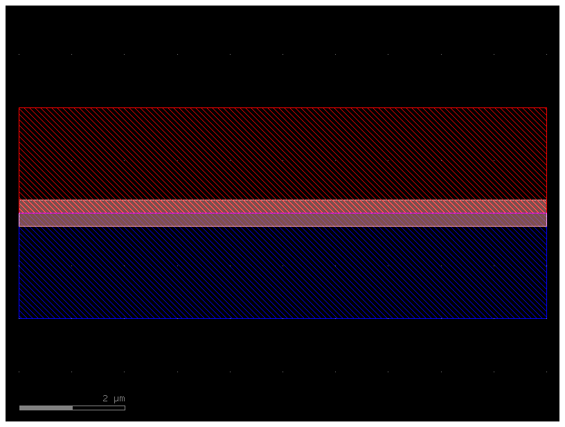
import gdsfactory as gf
from gdsfactory.cross_section import CrossSection, cross_section, xsection
from gdsfactory.typings import LayerSpec


@xsection
def pin(
    width: float = 0.5,
    layer: LayerSpec = "WG",
    radius: float = 10.0,
    radius_min: float = 5,
    layer_p: LayerSpec = (21, 0),
    layer_n: LayerSpec = (20, 0),
    width_p: float = 2,
    width_n: float = 2,
    offset_p: float = 1,
    offset_n: float = -1,
    **kwargs,
) -> CrossSection:
    """Return PIN cross_section."""
    sections = (
        (layer_p, offset_p - width_p / 2, offset_p + width_p / 2),
        (layer_n, offset_n - width_n / 2, offset_n + width_n / 2),
    )

    return cross_section(
        width=width,
        layer=layer,
        radius=radius,
        radius_min=radius_min,
        sections=sections,
        **kwargs,
    )
c = gf.components.straight(cross_section=pin)
c.plot()
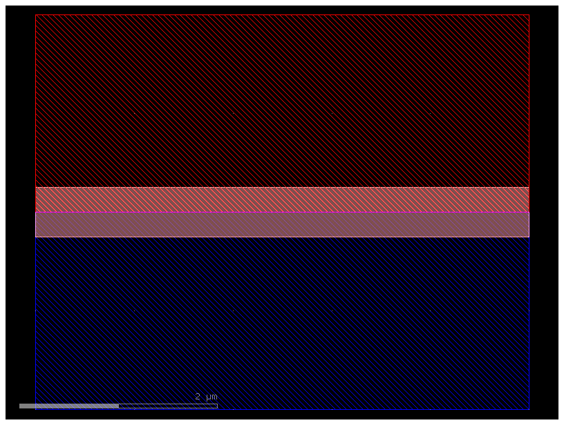
pin5 = gf.components.straight(cross_section=pin, length=5)
pin5.plot()
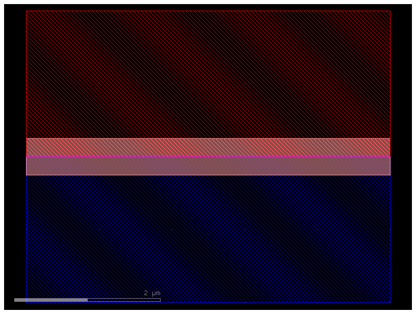
pin5 = gf.components.straight(cross_section="pin", length=5)
pin5.plot()
Finally, you can also pass the dictionary (dict) of most components that define the cross-section.
# Create our first cross-section
s0 = ((1, 0), 0 - 0.5 / 2, 0 + 0.5 / 2)
s1 = ((3, 0), 0 - 0.2 / 2, 0 + 0.2 / 2)
x1 = gf.cross_section.cross_section(width=None, sections=(s0, s1))

# Create the second cross-section that we want to transition to.
s0 = ((1, 0), 0 - 0.5 / 2, 0 + 0.5 / 2)
s1 = ((3, 0), 0 - 3.0 / 2, 0 + 3.0 / 2)
x2 = gf.cross_section.cross_section(width=None, sections=(s0, s1))

# To show the cross-sections, let us create two paths and create components by extruding them.
p1 = gf.path.straight(length=5)
p2 = gf.path.straight(length=5)
wg1 = gf.path.extrude(p1, x1)
wg2 = gf.path.extrude(p2, x2)

# Place both cross-section components and quickplot them.
c = gf.Component()
wg1ref = c << wg1
wg2ref = c << wg2
wg2ref.movex(7.5)

# Create the transitional cross-section.
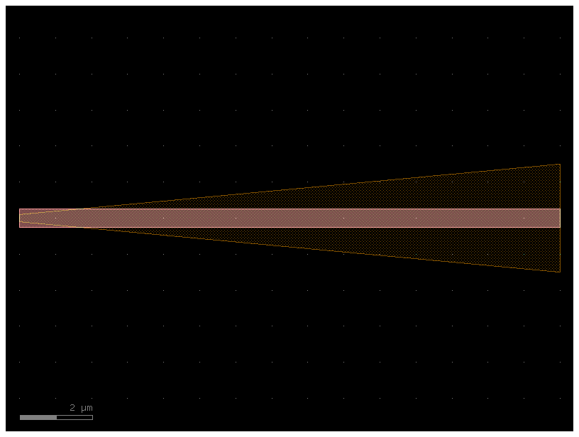
xtrans = gf.path.transition(cross_section1=x1, cross_section2=x2, width_type="linear")
# Create a path for the transitional cross-section to follow.
p3 = gf.path.straight(length=15, npoints=100)

# Use the transitional cross-section to create a component.
straight_transition = gf.path.extrude_transition(p3, xtrans)
straight_transition.plot()
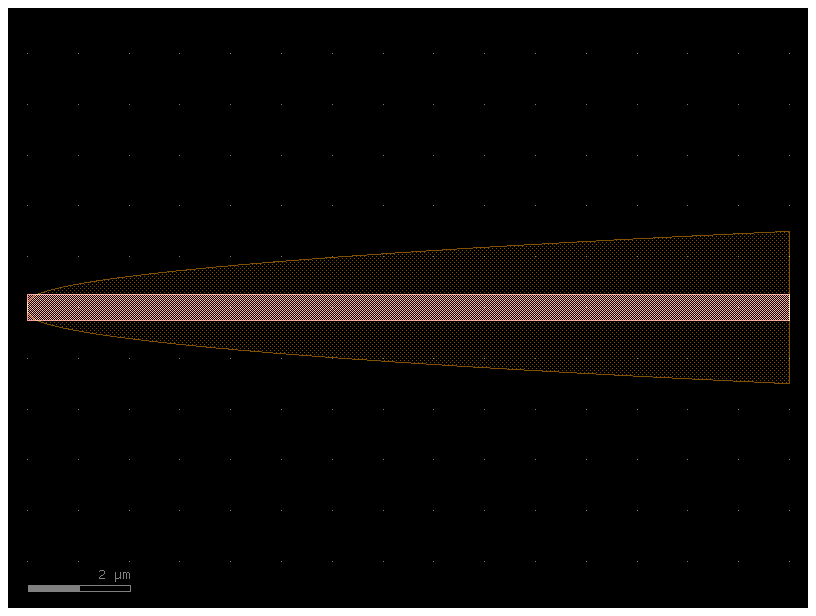
xtrans = gf.path.transition(
    cross_section1=x1, cross_section2=x2, width_type="parabolic"
)

p3 = gf.path.straight(length=15, npoints=100)


straight_transition = gf.path.extrude_transition(p3, xtrans)
straight_transition.plot()
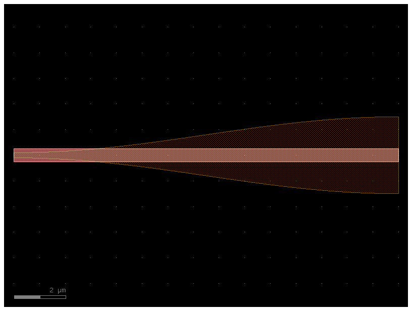
xtrans = gf.path.transition(cross_section1=x1, cross_section2=x2, width_type="sine")
p3 = gf.path.straight(length=15, npoints=100)


straight_transition = gf.path.extrude_transition(p3, xtrans)
straight_transition.plot()
s = straight_transition.to_3d()
s.show()
Symmetric and asymmetric profiles
gf.SymmetricCrossSection and gf.AsymmetricCrossSection are aliases for
kfactory.DCrossSection and kfactory.DAsymmetricCrossSection. Both accept
physical LayerInfo objects and use micrometers. Their common runtime union
is gf.CrossSection; it is not a constructor.
The factory snaps each strip edge independently before choosing the type. At a 1 nm DBU, a centered nominal width of 0.501 µm becomes 0.502 µm. An actual odd-DBU span, or an off-center strip, needs the asymmetric type.
xs_centered = gf.cross_section.cross_section(width=0.501, layer="WG")
xs_odd = gf.cross_section.cross_section(width=None, sections=[("WG", -0.250, 0.251)])
assert isinstance(xs_centered, gf.SymmetricCrossSection)
assert isinstance(xs_odd, gf.AsymmetricCrossSection)
assert xs_centered.width == 0.502
assert xs_odd.width == 0.501
xs_odd.get_sections()
(DCrossSectionLayer(layer=WG (1/0), section_min=-0.25, section_max=0.251),)
You can also construct a kfactory profile directly. Symmetric enclosure bands
are measured from the core edges; the factory's auxiliary tuples instead use
absolute transverse bounds. get_sections() resolves either representation
to absolute bounds, with the main strip first.
xs_direct = gf.SymmetricCrossSection(
    kcl=gf.kcl,
    width=0.8,
    layer=gf.get_layer_info("WG"),
    sections=[(gf.get_layer_info("SLAB90"), 3.0)],
    radius=10,
    radius_min=5,
)
assert isinstance(xs_direct, gf.CrossSection)
slab = xs_direct.get_sections()[1]
assert (slab.section_min, slab.section_max) == (-3.4, 3.4)
gf.path.straight(10).extrude(xs_direct).plot()
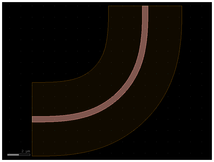
bbox_layers vs cladding_layers
For extruding waveguides you have two options:
- bbox_layers for squared bounding box.
- cladding_layers for extruding a layer that follows the shape of the path.
xs_bbox = gf.cross_section.cross_section(bbox_layers=((3, 0),), bbox_offsets=(3,))
w1 = gf.components.bend_euler(cross_section=xs_bbox, radius=10)
w1.plot()
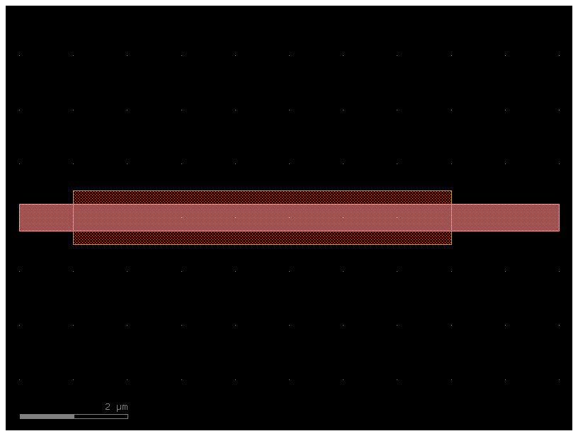
xs_clad = gf.cross_section.cross_section(cladding_layers=[(3, 0)], cladding_offsets=[3])
w2 = gf.components.bend_euler(cross_section=xs_clad, radius=10)
w2.plot()
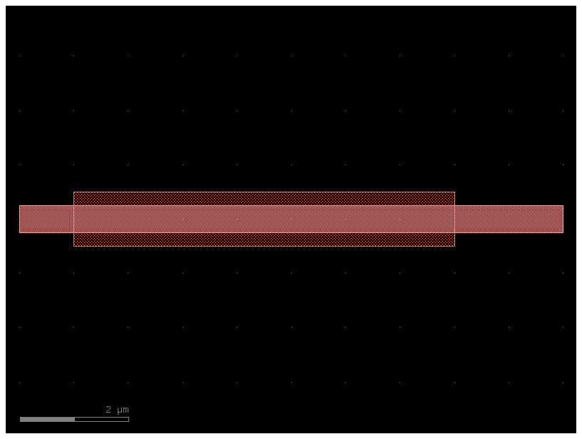
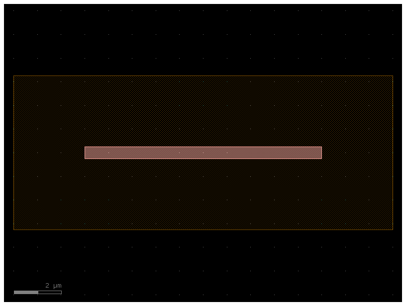
A profile stores bbox padding, but extrude() draws it only when
add_bbox=True. Component factories such as straight and bend_euler
request bbox drawing themselves. Cladding follows the path during ordinary
extrusion; bbox padding encloses the emitted geometry instead.
path = gf.path.straight(10)
bare = path.extrude(xs_bbox)
padded = path.extrude(xs_bbox, add_bbox=True)
bbox_layer = gf.get_layer((3, 0))
assert bare.dbbox(bbox_layer).empty()
assert padded.dbbox(bbox_layer) == gf.kdb.DBox(-3, -3.25, 13, 3.25)
padded.plot()
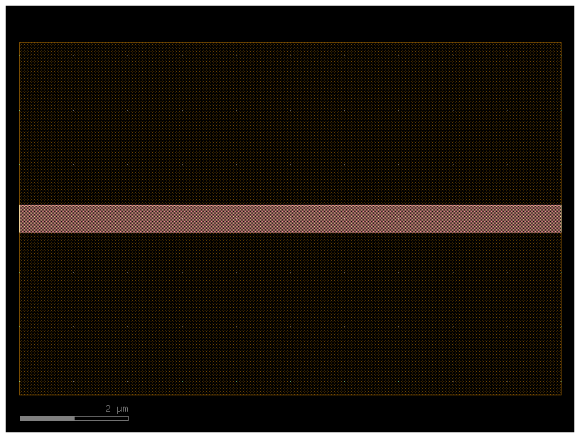
For manually assembled geometry, call xs.add_bbox(component) directly.
ref can select a layer, a Box/DBox, or an instance, but not a cell.
The profile, target and instance must share the same KCLayout.
Overrides such as left=0 keep selected edges unpadded.
Real cells with pending virtual instances report approximate bounds and warn:
call insert_vinsts() before adding a bbox when exact materialized bounds are
needed. Virtual cells (ComponentAllAngle) handle virtual instances normally.
assembly = gf.Component()
reference = assembly << bare
xs_bbox.add_bbox(assembly, ref=reference, left=0, right=0)
assert assembly.dbbox(bbox_layer) == gf.kdb.DBox(0, -3.25, 10, 3.25)
assembly.plot()
Profiles survive file round trips
Port metadata carries the complete kfactory profile, including auxiliary strips, radii and bbox padding. Keep metadata enabled when writing GDS/OAS. Reading into a different layout demonstrates that no gdsfactory cross-section factory registry is needed to reconstruct it.
import pathlib
import tempfile

import kfactory as kf

with tempfile.TemporaryDirectory() as directory:
    for suffix in ("gds", "oas"):
        filename = pathlib.Path(directory) / f"profile.{suffix}"
        padded.write(filename)
        restored_layout = kf.KCLayout(f"tutorial_read_{suffix}")
        restored_layout.read(filename)
        top = restored_layout.layout.top_cell()
        restored = restored_layout[top.cell_index()].to_dtype()
        assert restored.ports["o1"].cross_section.base == xs_bbox.base
        assert restored.ports["o1"].dcplx_trans == padded.ports["o1"].dcplx_trans
        assert restored.dbbox() == padded.dbbox()
This reads the bbox metadata and shapes; it does not call add_bbox() again.
To compare layer geometry across layouts, resolve layer indices separately in
each layout: identical integer layer indices need not mean identical layers.
Insets
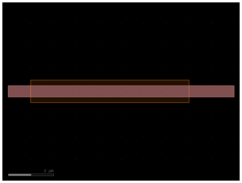
Pass insets={section_index: (start, end)} to extrude() to trim individual strips along the path. Ports follow the trimmed endpoints. Insets and port choices are not stored in the profile.
xs = gf.cross_section.cross_section(
    layer="WG", width=0.5, sections=[("HEATER", -0.5, 0.5)]
)
c = gf.path.straight(10).extrude(
    xs, insets={1: (1, 2)}, ports={0: ("o1", "o2", "optical")}
)
c.plot()
xs = gf.cross_section.cross_section(
    layer="WG", width=0.5, sections=[("HEATER", -0.5, 0.5)]
)
c = gf.path.straight(10).extrude(
    xs,
    insets={1: (1, 2)},
    ports={0: ("o1", "o2", "optical"), 1: ("e1", "e2", "electrical")},
)
c.plot()