Shapes and generic cells

gdsfactory provides some generic parametric cells in gf.components that you can customize for your application.

Basic shapes

Rectangle

To create a simple rectangle, there are two functions:

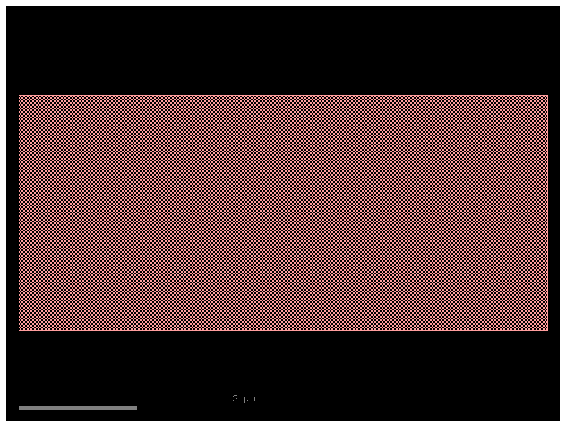
gf.components.rectangle() can create a basic rectangle:

import gdsfactory as gf



gf.gpdk.PDK.activate()
r1 = gf.components.rectangle(size=(4.5, 2), layer=(1, 0))
r1.plot()

png

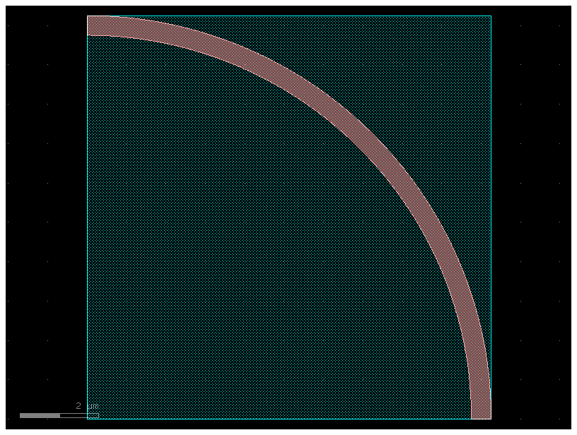
gf.components.bbox() can also create a rectangle based on a bounding box. This is useful if you want to create a rectangle which precisely surrounds a piece of existing geometry. For example, if we have an arc geometry and we want to define a box around it, we can use gf.components.bbox():

c = gf.Component()
arc = c << gf.components.bend_circular(radius=10, width=0.5, angle=90, layer=(1, 0))
arc.rotate(90)

# Draw a rectangle around the arc we created by using the arc's bounding box.
rect = c << gf.components.bbox(arc, layer=(2, 0))
c.plot()

png

Cross

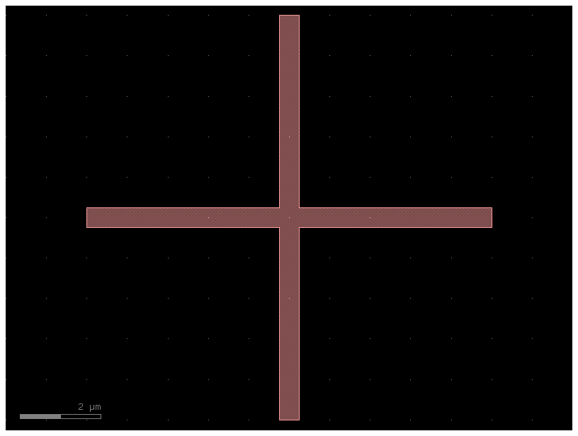
The gf.components.cross() function creates a cross structure:

c = gf.components.cross(length=10, width=0.5, layer=(1, 0))
c.plot()

png

Ellipse

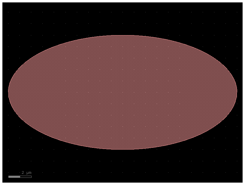
The gf.components.ellipse() function creates an ellipse by defining the major and minor radii:

c = gf.components.ellipse(radii=(10, 5), angle_resolution=2.5, layer=(1, 0))
c.plot()

png

Circle

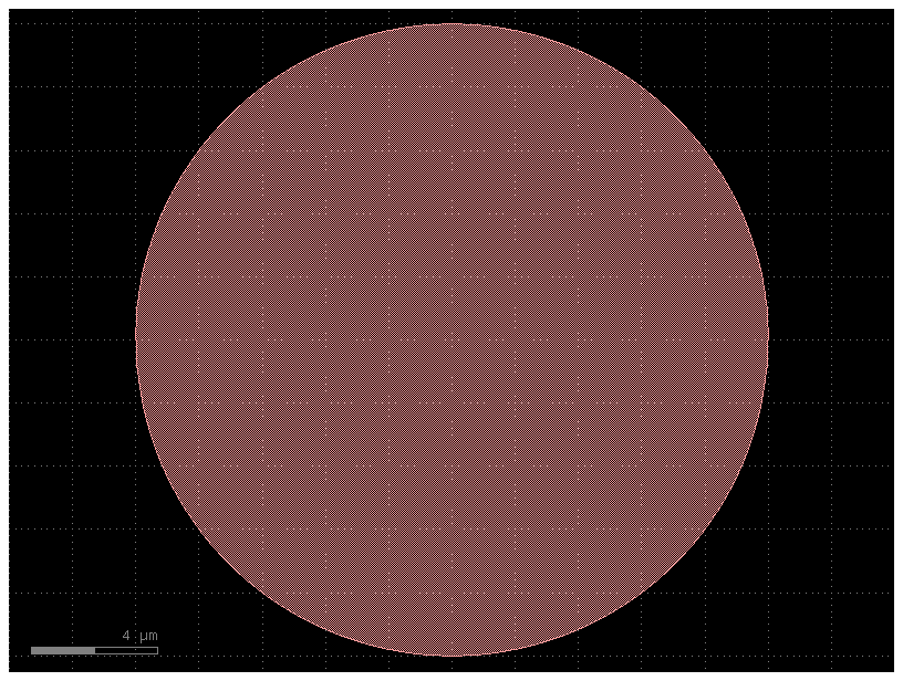
The gf.components.circle() function creates a circle:

c = gf.components.circle(radius=10, angle_resolution=2.5, layer=(1, 0))
c.plot()

png

Ring

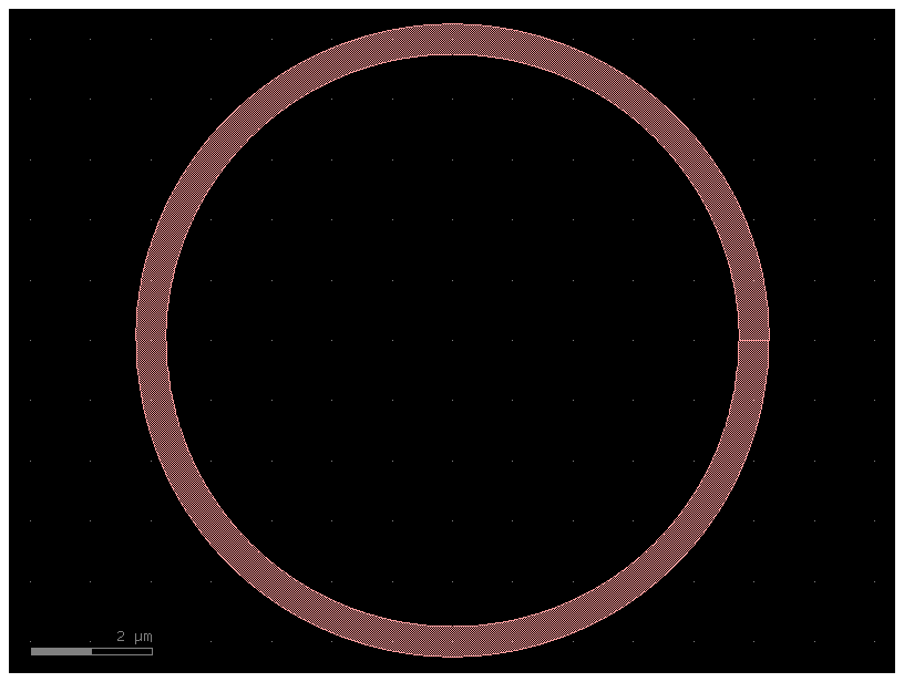
The gf.components.ring() function creates a ring. The radius refers to the center radius of the ring structure (halfway between the inner and outer radius).

c = gf.components.ring(radius=5, width=0.5, angle_resolution=2.5, layer=(1, 0))
c.plot()

png

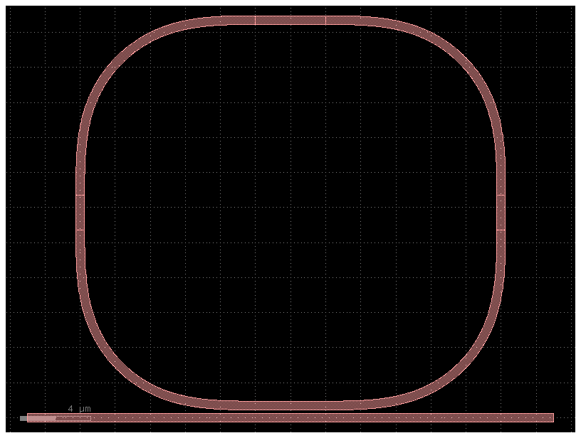
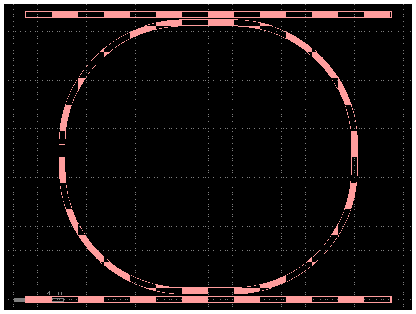
c = gf.components.ring_single(gap=0.2, radius=10, length_x=4, length_y=2)
c.plot()

png

import gdsfactory as gf

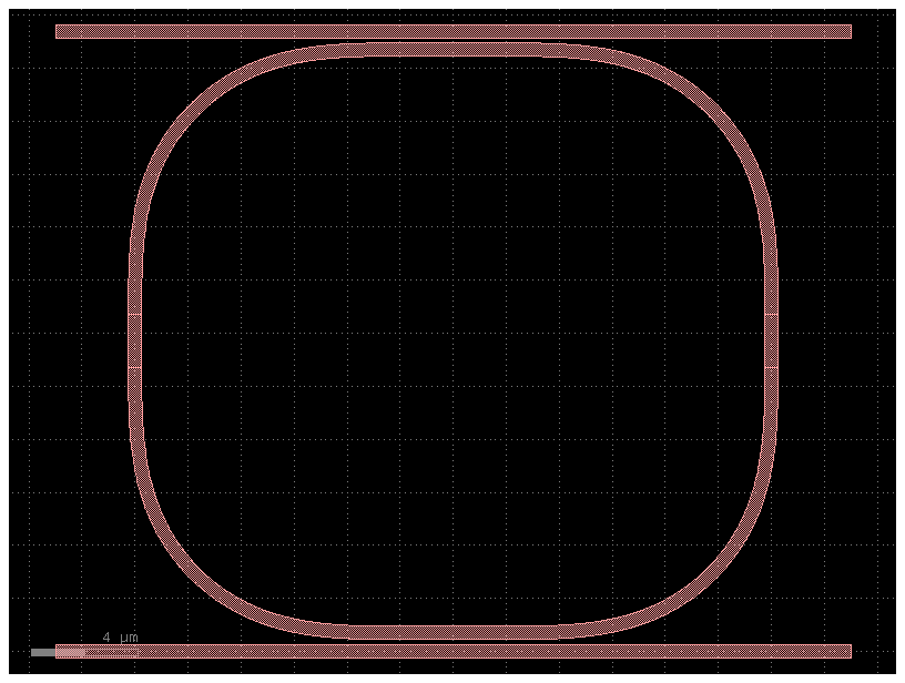
c = gf.components.ring_double(gap=0.2, radius=10, length_x=4, length_y=2)
c.plot()

png

c = gf.components.ring_double(
    gap=0.2,
    radius=10,
    length_x=4,
    length_y=2,
    bend=gf.components.bend_circular,
)
c.plot()

png

Bend circular

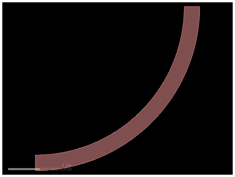
The gf.components.bend_circular() function creates an arc. The radius refers to the center radius of the arc (halfway between the inner and outer radius).

c = gf.components.bend_circular(
    radius=5.0, width=0.5, angle=90, npoints=720, layer=(1, 0)
)
c.plot()

png

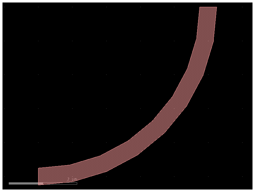
You can control the point spacing of bends using angular_step (degrees between consecutive points) or npoints. For a target distance between points, calculate the angular step from the radius: angular_step = spacing / radius * (180 / pi). For example, 1 um spacing on a 5 um radius bend gives angular_step ≈ 11.5°.

import numpy as np

radius = 5.0
target_spacing_um = 1.0  # 1 um between points
angular_step = target_spacing_um / radius * (180 / np.pi)
print(f"angular_step = {angular_step:.2f} degrees for {target_spacing_um} um spacing")

c = gf.components.bend_circular(
    radius=radius, width=0.5, angle=90, angular_step=angular_step, layer=(1, 0)
)
first_layer = next(iter(c.get_polygons()))
print(f"Number of polygon points: {c.get_polygons()[first_layer][0].num_points()}")
c.plot()

angular_step = 11.46 degrees for 1.0 um spacing
Number of polygon points: 18

png

Bend euler

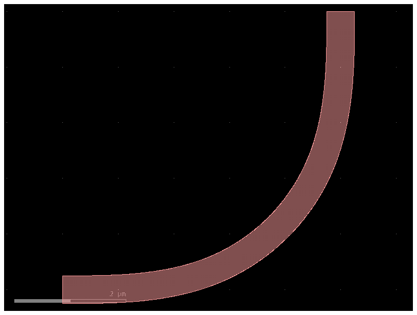
The gf.components.bend_euler() function creates an adiabatic bend in which the bend radius changes gradually. Euler bends have lower loss than circular bends.

c = gf.components.bend_euler(radius=5.0, width=0.5, angle=90, npoints=720, layer=(1, 0))
c.plot()

png

Similarly, you can use angular_step with Euler bends. Note that angular_step and npoints are mutually exclusive.

radius = 5.0
target_spacing_um = 1.0
angular_step = target_spacing_um / radius * (180 / np.pi)

c = gf.components.bend_euler(
    radius=radius, width=0.5, angle=90, angular_step=angular_step, layer=(1, 0)
)
first_layer = next(iter(c.get_polygons()))
print(f"Number of polygon points: {c.get_polygons()[first_layer][0].num_points()}")
c.plot()

Number of polygon points: 14

png

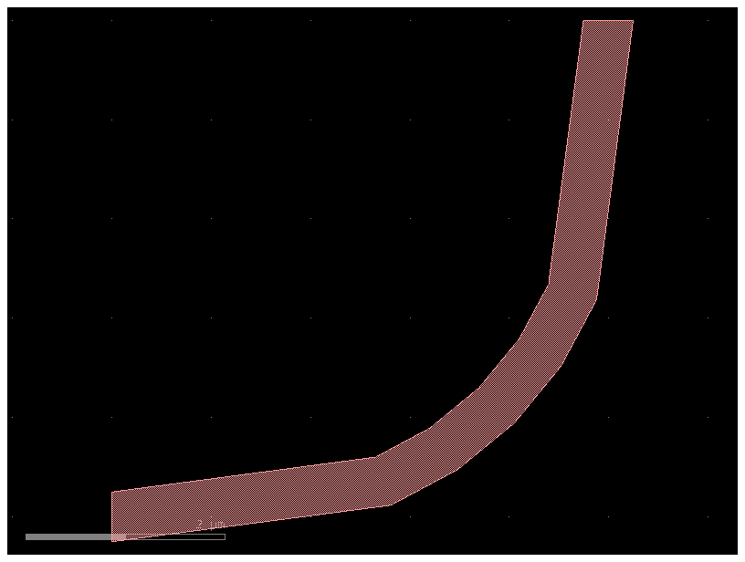
You can also set the default point density globally via PDK.bend_points_distance (in um). Smaller values produce denser points. Set this before creating bends, as cell caching captures the value at creation time.

PDK = gf.get_active_pdk()
PDK.bend_points_distance = 0.1  # 100 nm spacing between points

c = gf.components.bend_euler(radius=5.0, width=0.5, angle=90, layer=(1, 0))
first_layer = next(iter(c.get_polygons()))
print(f"Number of polygon points: {c.get_polygons()[first_layer][0].num_points()}")
c.plot()

Number of polygon points: 70

png

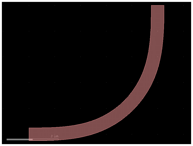
PDK.bend_points_distance = 20e-3  # reset to default 20 nm

Tapers

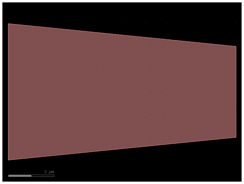
gf.components.taper()is defined by setting its length as well as its start and end length. It has two ports, 1 and 2, on either end, allowing you to easily connect it to other structures.

c = gf.components.taper(length=10, width1=6, width2=4, port=None, layer=(1, 0))
c.plot()

png

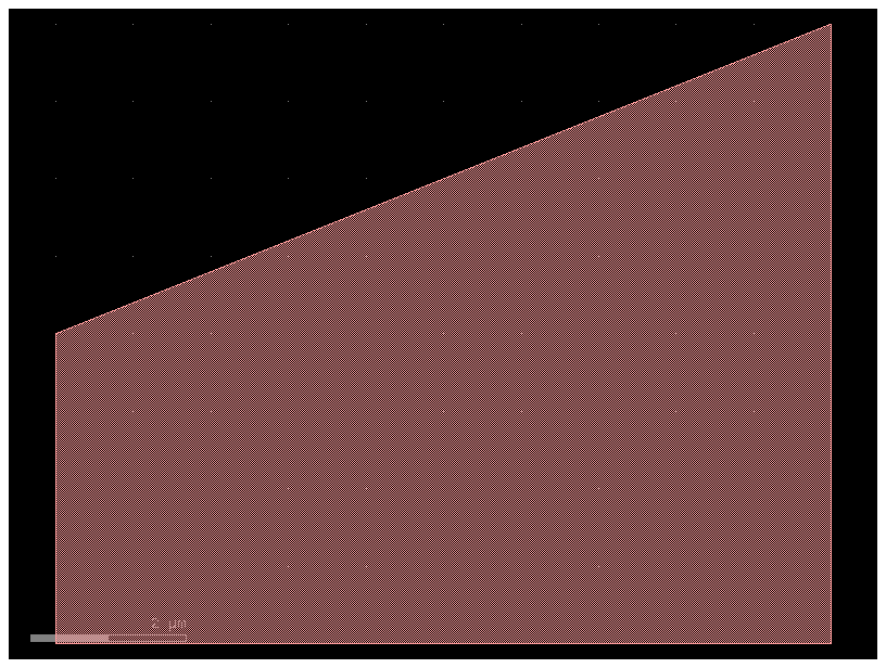
gf.components.ramp() is a structure is similar to taper() except it is asymmetric. It also has two ports, 1 and 2, on either end.

c = gf.components.ramp(length=10, width1=4, width2=8, layer=(1, 0))
c.plot()

png

Common compound shapes

The gf.components.L() function creates a "L" shape with ports on either end named 1 and 2.

c = gf.components.L(width=7, size=(10, 20), layer=(1, 0))
c.plot()

png

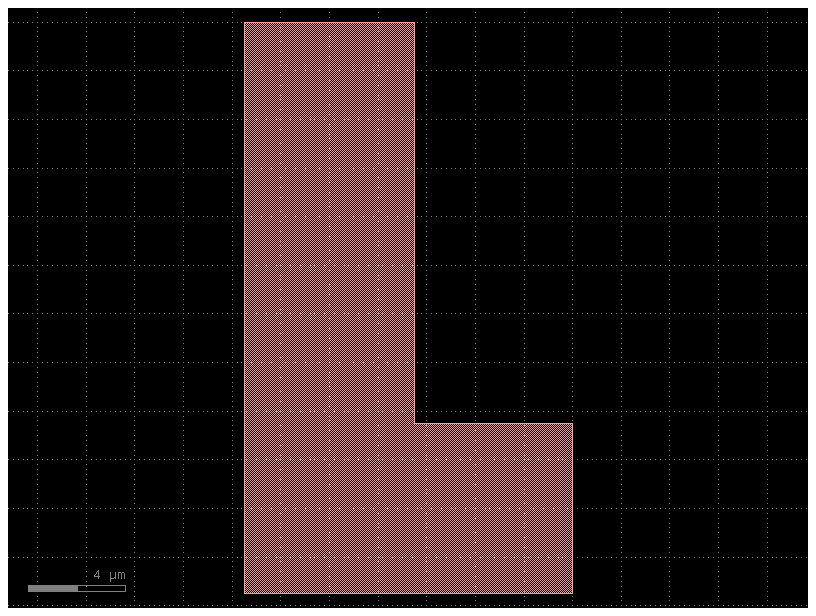
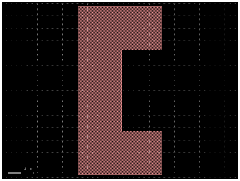
The gf.components.C() function creates a "C" shape with ports on either end named 1 and 2.

c = gf.components.C(width=7, size=(10, 20), layer=(1, 0))
c.plot()

png

Text

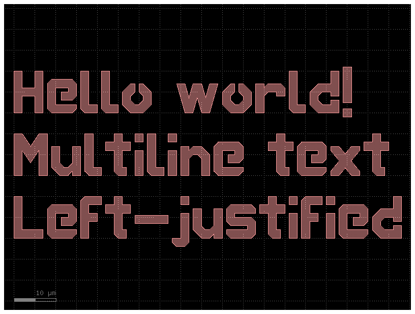
Gdsfactory has an implementation of the DEPLOF font with the majority of english ASCII characters represented (thanks to PHIDL)

c = gf.components.text(
    text="Hello world!\nMultiline text\nLeft-justified",
    size=10,
    justify="left",
    layer=(1, 0),
)
c.plot()
# The justify parameter needs to be 'left', 'center', or 'right',
# because those are the standard text alignment options that determine how multiple lines of text are positioned relative to each other.

png

Lithography Structures

Step-resolution

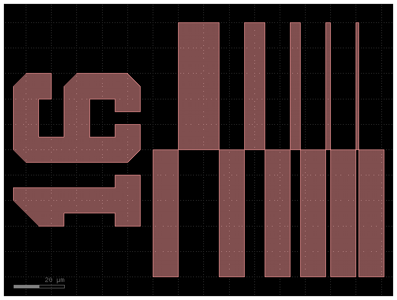
The gf.components.litho_steps() function creates a lithographic test structure that is useful for measuring the resolution of photoresist or electron-beam resists. It provides both positive-tone and negative-tone resolution tests.

c = gf.components.litho_steps(
    line_widths=(1, 2, 4, 8, 16), line_spacing=10, height=100, layer=(1, 0)
)
c.plot()

png

Calipers (inter-layer alignment)

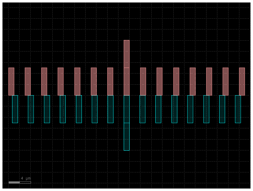
The gf.components.litho_calipers() function is used to detect offsets in multilayer fabrications. It creates a set of two notches on different layers. When a fabrication error/offset occurs, it is easy to detect the magnitude of the offset because both center-notches are no longer aligned.

D = gf.components.litho_calipers(
    notch_size=(1, 5),
    notch_spacing=2,
    num_notches=7,
    offset_per_notch=0.1,
    row_spacing=0,
    layer1=(1, 0),
    layer2=(2, 0),
)
D.plot()

png

Paths

See Path tutorial for more details -- this is just an enumeration of the available built-in Path functions

Circular arc

P = gf.path.arc(radius=10, angle=135, npoints=720)
f = P.plot()

png

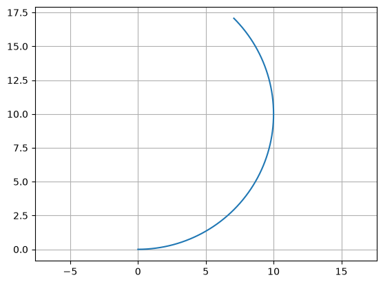
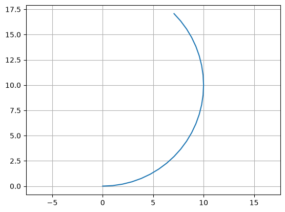
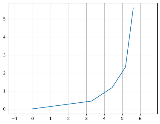
You can use angular_step instead of npoints to define the angular resolution in degrees. To get 1 um spacing, calculate angular_step = spacing / radius * (180 / pi).

import numpy as np

radius = 10
angular_step = 1.0 / radius * (180 / np.pi)  # 1 um spacing
P = gf.path.arc(radius=radius, angle=135, angular_step=angular_step)
f = P.plot()

png

Straight

import gdsfactory as gf

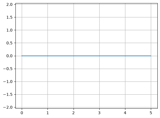
P = gf.path.straight(length=5, npoints=100)
f = P.plot()

png

Euler curve

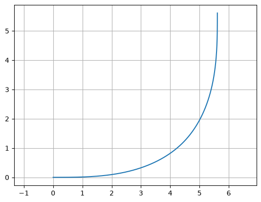
Also known as a straight-to-bend, clothoid, racetrack, or track transition, this path tapers adiabatically from straight to curved. Often used to minimize losses in photonic straights. If p < 1.0, it will create a "partial euler" curve as described in Vogelbacher et. al. https://dx.doi.org/10.1364/oe.27.031394.
If the use_eff argument is false, radius corresponds to minimum radius of curvature of the bend. If use_eff is true, radius corresponds to the "effective" radius of the bend-- The curve will be scaled such that the endpoints match an arc with parameters radius and angle.

P = gf.path.euler(radius=3, angle=90, p=1.0, use_eff=False, npoints=720)
f = P.plot()

png

radius = 3
angular_step = 1.0 / radius * (180 / np.pi)  # 1 um spacing
P = gf.path.euler(radius=radius, angle=90, p=1.0, use_eff=False, angular_step=angular_step)
f = P.plot()

png

Smooth path from waypoints

import numpy as np

import gdsfactory as gf

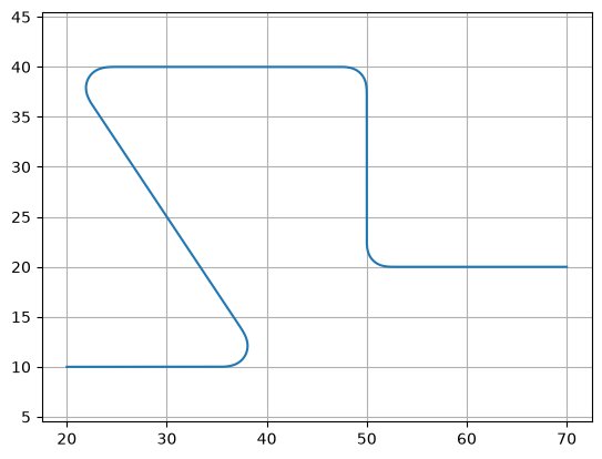
points = np.array([(20, 10), (40, 10), (20, 40), (50, 40), (50, 20), (70, 20)])

P = gf.path.smooth(
    points=points,
    radius=2,
    bend=gf.path.euler,
    use_eff=False,
)
f = P.plot()

png

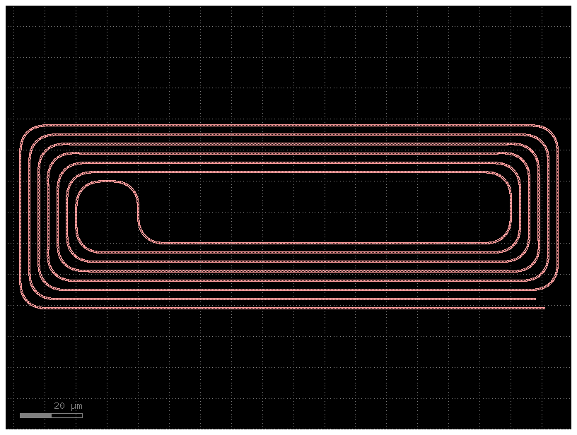
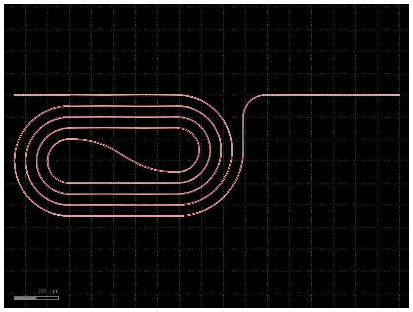
Delay spiral

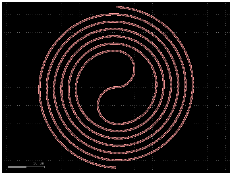
A delay spiral is a long optical waveguide coiled into a spiral shape on a photonic integrated circuit. Its purpose is to create a significant time delay for an optical signal within a very compact area.

c = gf.components.spiral_double()
c.plot()

png

c = gf.components.spiral()
c.plot()

png

c = gf.components.spiral_racetrack_fixed_length()
c.plot()

png

Useful contact pads / connectors

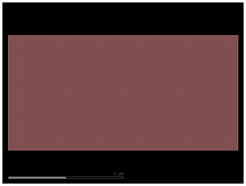
These functions are common shapes with ports, often used to make contact pads.

c = gf.components.compass(size=(4, 2), layer=(1, 0))
c.plot()

png

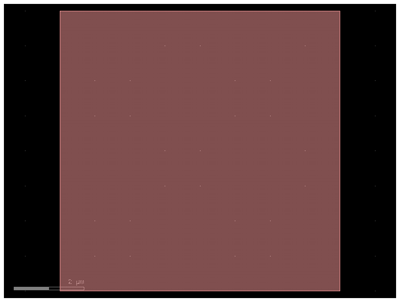
c = gf.components.nxn(north=3, south=4, east=0, west=0)
c.plot()

png

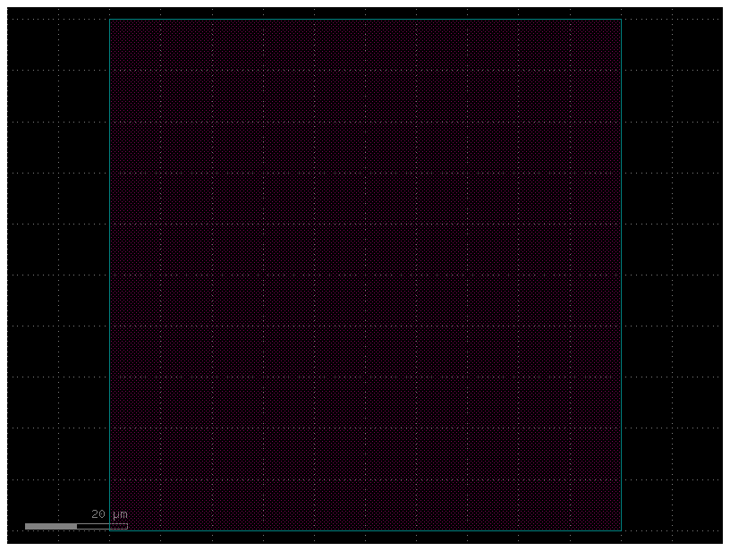
c = gf.components.pad()
c.plot()

png

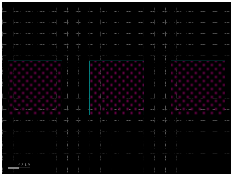
c = gf.components.pad_array90(columns=3)
c.plot()

png

Chip / die template

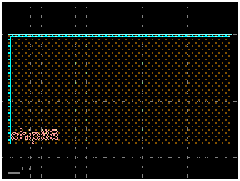
import gdsfactory as gf

c = gf.components.die(
    size=(10000, 5000),  # Size of the die.
    street_width=100,  # Width of corner marks for die-sawing.
    street_length=1000,  # Length of corner marks for die-sawing.
    die_name="chip99",  # Label text.
    text_size=500,  # Label text size.
    text_location="SW",  # Label text compass location e.g. 'S', 'SE', 'SW'
    layer=(2, 0),
    bbox_layer=(3, 0),
)
c.plot()

png

Optimal superconducting curves

The following structures are meant to reduce "current crowding" in superconducting thin-film structures (such as superconducting nanowires). They are the result of conformal mapping equations derived in Clem, J. & Berggren, K. "Geometry-dependent critical currents in superconducting nanocircuits." Phys. Rev. B 84, 1–27 (2011).

import gdsfactory as gf

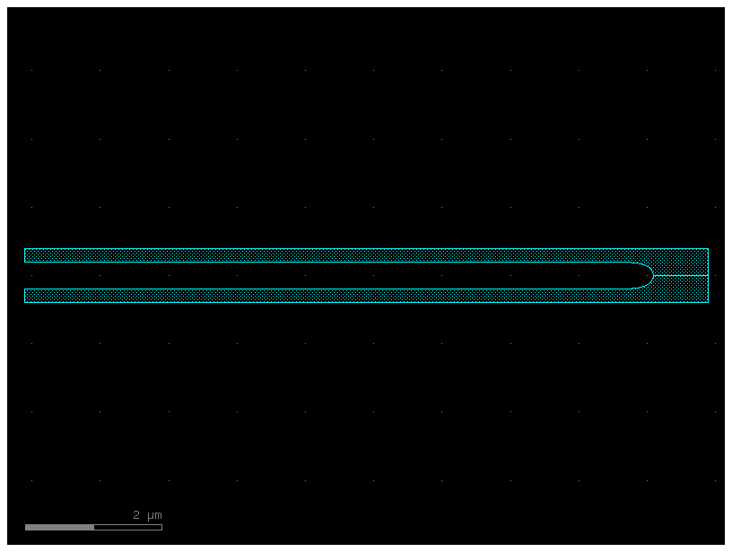
# This code creates a compact, U-shaped "hairpin" delay line with bends that are optimized for low loss.
c = gf.components.optimal_hairpin(
    width=0.2, pitch=0.6, length=10, turn_ratio=4, num_pts=50, layer=(2, 0)
)
c.plot()

png

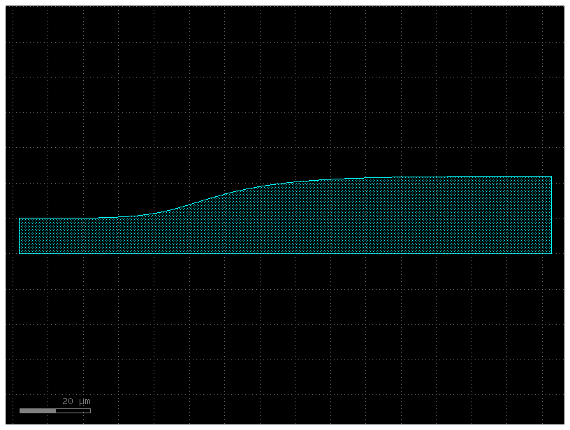
# This code creates a taper, which is a waveguide section that smoothly transitions between two different widths.
# The optimal_step component is special because its shape is mathematically optimized to be adiabatic, minimizing light loss and back-reflections.
c = gf.components.optimal_step(
    start_width=10, # Defines the initial width of the taper.
    end_width=22, # Defines the final width of the taper.

    # num_pts=50: This sets the number of points used to define the optimized S-curve. A higher number results in a smoother, more finely detailed curve.
    num_pts=50,

    # This is the width tolerance. It defines how close the optimization algorithm must get to the target end_width.
    # A smaller value results in a more precise, but potentially longer, taper.
    width_tol=1e-3,

    # This factor adjusts the "aggressiveness" of the S-curve.
    # A larger value creates a more gradual, less crowded transition at the start and end of the taper.
    anticrowding_factor=1.2,

    # This parameter creates a one-sided taper. One edge of the taper will be a straight line, while the other will have the optimized S-curve.
    # If True, both sides would curve symmetrically.
    symmetric=False,
    layer=(2, 0),
)
c.plot()

png

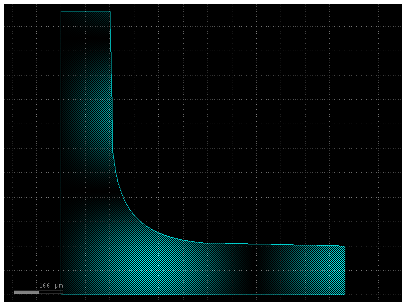
c = gf.components.optimal_90deg(width=100.0, num_pts=15, length_adjust=1, layer=(2, 0))
c.plot()

png

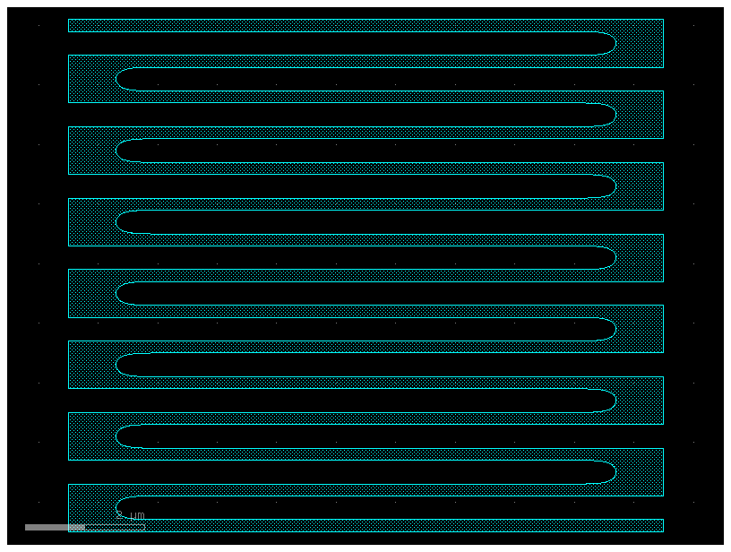
# This code creates a Superconducting Nanowire Single-Photon Detector (SNSPD), a specialized component designed to detect single photons of light.
c = gf.components.snspd(
    wire_width=0.2,
    wire_pitch=0.6,
    size=(10, 8), # The overall dimensions of the meandered detector area are 10x8 µm.
    num_squares=None, # num_squares=None means that the size of the component is being defined by the size parameter.
    turn_ratio=4, # Controls the shape of the 180-degree bends in the meander(Clojure/Clojurescript library).
    terminals_same_side=False, # The input and output terminals will be on opposite sides of the detector.
    layer=(2, 0),
)
c.plot()

png

Generic library

gdsfactory comes with a generic library that you can customize to your needs or even modify the internal code to create the components that you need.