Analytical process simulation¶

The simplest (and quickest) process simulation involves analytical implant tables, followed by broadening of the profile according to a tabulated diffusion coefficient.

The implant module of gdsfactory tabulates these expressions for silicon and common implants, and allows you to import them to TCAD solvers.

For more exact implant simulation, see the numerical implantation and numerical diffusion modules.

References:

[1] Selberherr, S. (1984). Process Modeling. In: Analysis and Simulation of Semiconductor Devices. Springer, Vienna. https://doi.org/10.1007/978-3-7091-8752-4_3

import matplotlib.pyplot as plt
import numpy as np

from gplugins.process.diffusion import D, silicon_diffused_gaussian_profile
from gplugins.process.implant_tables import (
    depth_in_silicon,
    silicon_gaussian_profile,
    silicon_skewed_gaussian_profile,
    skew_in_silicon,
    straggle_in_silicon,
)

Gaussian profile¶

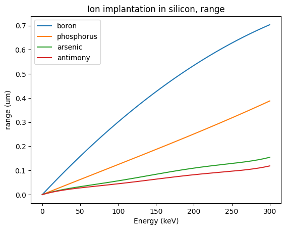
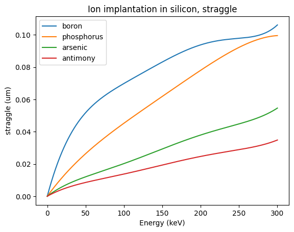
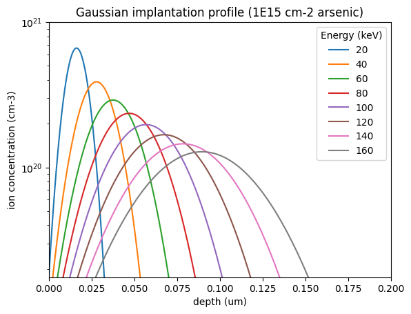
The simplest approximation to an implantation profile only considers the range (mean) and straggle (standard deviation) of the ion distribution:

energies = np.linspace(0, 300, 1000)  # keV

for dopant in ["boron", "phosphorus", "arsenic", "antimony"]:
    plt.plot(energies, depth_in_silicon[dopant](energies), label=dopant)

plt.xlabel("Energy (keV)")
plt.ylabel("range (um)")
plt.legend(loc="best")
plt.title("Ion implantation in silicon, range")

Text(0.5, 1.0, 'Ion implantation in silicon, range')

png

for dopant in ["boron", "phosphorus", "arsenic", "antimony"]:
    plt.plot(energies, straggle_in_silicon[dopant](energies), label=dopant)

plt.xlabel("Energy (keV)")
plt.ylabel("straggle (um)")
plt.legend(loc="best")
plt.title("Ion implantation in silicon, straggle")

Text(0.5, 1.0, 'Ion implantation in silicon, straggle')

png

energies = [20, 40, 60, 80, 100, 120, 140, 160]
z = np.linspace(0, 0.25, 1000)


lower_lim = 0
for E in energies:
    c = silicon_gaussian_profile("arsenic", dose=1e15, E=E, z=z)
    plt.semilogy(z, c, label=E)
    if c[0] > lower_lim:
        lower_lim = c[0]

plt.xlabel("depth (um)")
plt.ylabel("ion concentration (cm-3)")
plt.ylim([lower_lim, 1e21])
plt.xlim([0, 0.2])
plt.title("Gaussian implantation profile (1E15 cm-2 arsenic)")
plt.legend(title="Energy (keV)")

<matplotlib.legend.Legend at 0x7fc822e3cd40>

png

Skewed Gaussian profile¶

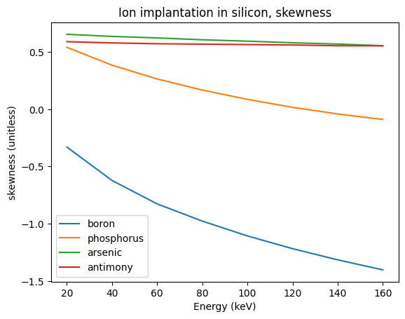
For more realistic results with nonzero skewness (we catalog the skews of [1], but your mileage may vary), two half-gaussians can better approximate the distribution:

for dopant in ["boron", "phosphorus", "arsenic", "antimony"]:
    plt.plot(energies, skew_in_silicon[dopant](energies), label=dopant)

plt.xlabel("Energy (keV)")
plt.ylabel("skewness (unitless)")
plt.legend(loc="best")
plt.title("Ion implantation in silicon, skewness")

Text(0.5, 1.0, 'Ion implantation in silicon, skewness')

png

energies = [20, 40, 60, 80, 100, 120, 140, 160]
z = np.linspace(0, 0.25, 1000)


lower_lim = 0
for E in energies:
    c = silicon_skewed_gaussian_profile("arsenic", dose=1e11, E=E, z=z)
    plt.semilogy(z, c, label=E)
    if c[0] > lower_lim:
        lower_lim = c[0]

plt.xlabel("depth (um)")
plt.ylabel("ion concentration (cm-2)")
plt.ylim([lower_lim, 1e18])
plt.xlim([0, 0.2])
plt.title("Joined half Gaussian implantation profile (|skew| <~ 1)")
plt.legend(title="Energy (keV)")

<matplotlib.legend.Legend at 0x7fc822b7e0f0>

png

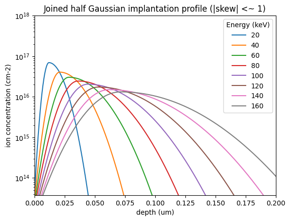
The above can be further improved by considering a Pearson IV distribution, or performing Monte-Carlo simulations of implantation.

Diffusion¶

Thermal treatment of the wafer to anneal implantation defects and activate the dopants results in rearrangement of the doping ions, and hence a change in doping profile. This is governed by the diffusivity of the species in the crystal:

Ts = np.linspace(800, 1100, 100)

for dopant in ["boron", "phosphorus", "arsenic", "antimony"]:
    plt.semilogy(Ts, D(dopant, Ts), label=dopant)

plt.xlabel("Temperature (C)")
plt.ylabel("Diffusivity (cm2 s-1)")
plt.title("Intrinsic diffusivity (n=p=ni)")
plt.legend()

<matplotlib.legend.Legend at 0x7fc8208f3770>

png

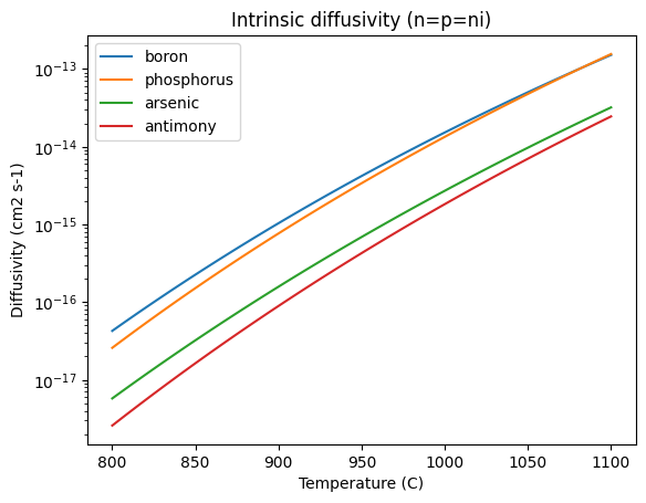
In this low-doping regime, the diffusivity can be taken as constant, and there exist an analytical solution for initially Gaussian doping profiles:

T = 1000  # C
dopant = "phosphorus"
dose = 1e12  # ions/cm2
E = 100  # keV
z = np.linspace(0, 0.6, 1000)

for t in [0, 60, 5 * 60, 10 * 60]:
    conc = silicon_diffused_gaussian_profile(
        dopant=dopant,
        dose=dose,
        E=E,
        t=t,
        T=T,
        z=z,
    )
    plt.plot(conc, label=t)
plt.title(f"{dopant} dose={dose:1.0e} ions/cm2, E={E}keV")
plt.xlabel("depth (um)")
plt.ylabel("ion concentration (cm-3)")
plt.legend(title=f"Diffusion time @ {T}C (s)")
plt.show()

png

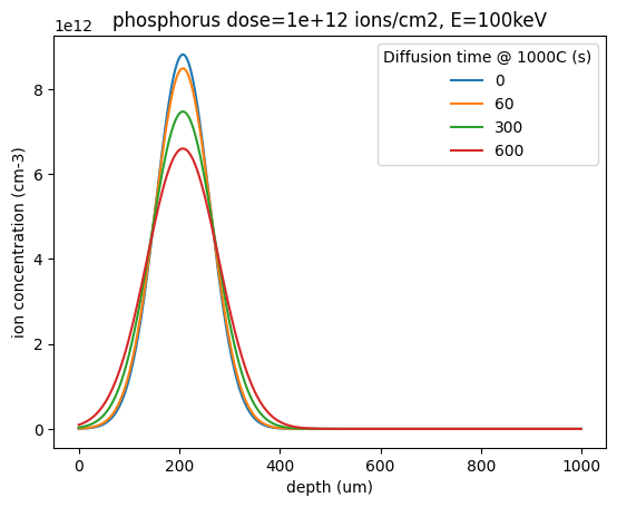
This can be extended to many dimensions.

Concentration-dependent diffusion¶

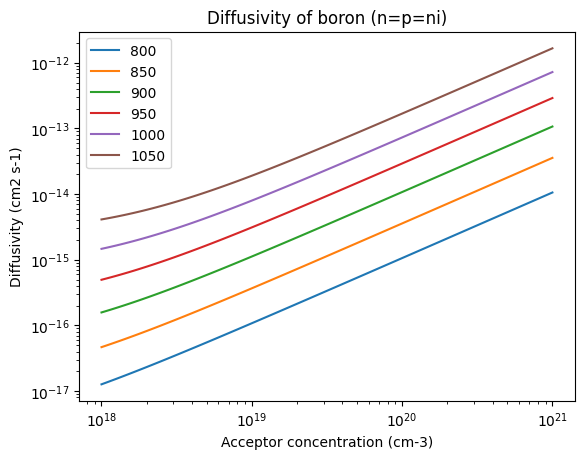
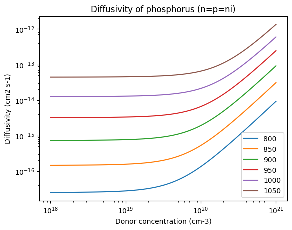
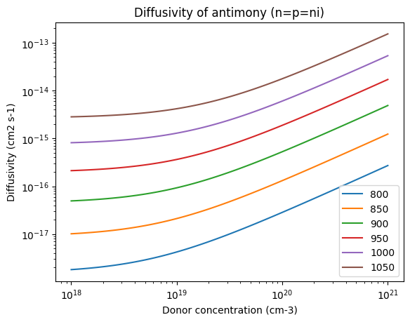
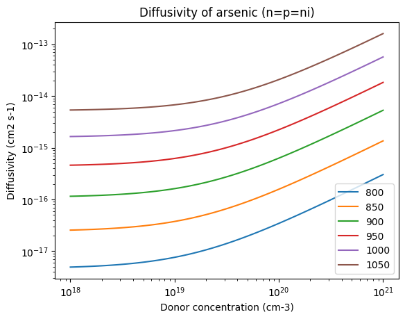
In general, especially at higher concentrations, diffusivity depends on concentration:

Ts = [800, 850, 900, 950, 1000, 1050]
conc = np.logspace(18, 21, 100)

for T in Ts:
    plt.loglog(conc, D("boron", T, n=conc, p=conc), label=T)

plt.xlabel("Acceptor concentration (cm-3)")
plt.ylabel("Diffusivity (cm2 s-1)")
plt.title("Diffusivity of boron (n=p=ni)")
plt.legend()

<matplotlib.legend.Legend at 0x7fc8205b25d0>

png

for T in Ts:
    plt.loglog(conc, D("phosphorus", T, n=conc, p=conc), label=T)

plt.xlabel("Donor concentration (cm-3)")
plt.ylabel("Diffusivity (cm2 s-1)")
plt.title("Diffusivity of phosphorus (n=p=ni)")
plt.legend()

<matplotlib.legend.Legend at 0x7fc82073eed0>

png

for T in Ts:
    plt.loglog(conc, D("antimony", T, n=conc, p=conc), label=T)

plt.xlabel("Donor concentration (cm-3)")
plt.ylabel("Diffusivity (cm2 s-1)")
plt.title("Diffusivity of antimony (n=p=ni)")
plt.legend()

<matplotlib.legend.Legend at 0x7fc8201e6630>

png

for T in Ts:
    plt.loglog(conc, D("arsenic", T, n=conc, p=conc), label=T)

plt.xlabel("Donor concentration (cm-3)")
plt.ylabel("Diffusivity (cm2 s-1)")
plt.title("Diffusivity of arsenic (n=p=ni)")
plt.legend()

<matplotlib.legend.Legend at 0x7fc820579280>

png

The most generic solution considers the local forms of these concentration-dependent diffusivities for the diffusion equation of each dopant, as well as the electrostatic potential, in a finite-element scheme.