Electrostatic simulations with Elmer
Here, we show how Elmer may be used to perform electrostatic simulations. For a given geometry, one needs to specify the terminals where to apply potential. The result is a Maxwell capacitance matrix. With no grounded conductor, the zero-flux outer boundary gives a floating network whose matrix rows sum to zero. For details on the physics, see [@smolic_capacitance_2021].
Installation
See Elmer FEM – Installation for installation or compilation instructions. Gplugins assumes ElmerSolver, ElmerSolver_mpi, and ElmerGrid are available in your PATH environment variable.
Alternatively, Singularity / Apptainer containers may be used. An example definition file is found at CSCfi/singularity-recipes and can be built with:
Afterwards, an easy install method is to add scripts to~/.local/bin (or elsewhere in PATH) calling the Singularity container for each of the necessary executables. For example, one may create a ElmerSolver_mpi file containing
Geometry, layer config and materials
from math import inf

import gdsfactory as gf
from gdsfactory.gpdk import LAYER, get_generic_pdk
from gdsfactory.technology import LayerStack
from gdsfactory.technology.layer_stack import LayerLevel
from meshwell.resolution import ConstantInField

from gplugins.elmer import run_capacitive_simulation_elmer

gf.config.rich_output()
PDK = get_generic_pdk()
PDK.activate()
We employ an example LayerStack used in superconducting circuits similar to [@marxer_long-distance_2023]. The stack carries an explicit vacuum layer: the driver needs a named background volume, and meshwell no longer accepts background_padding.
layer_stack = LayerStack(
    layers=dict(
        substrate=LayerLevel(
            layer=LAYER.WAFER,
            thickness=500,
            zmin=0,
            material="Si",
            mesh_order=99,
        ),
        bw=LayerLevel(
            layer=LAYER.WG,
            thickness=200e-3,
            zmin=500,
            material="Nb",
            mesh_order=2,
        ),
        vacuum=LayerLevel(
            layer=LAYER.WAFER,
            thickness=700,
            zmin=500,
            material="vacuum",
            mesh_order=100,
        ),
    )
)
material_spec = {
    "Si": {"relative_permittivity": 11.45},
    "Nb": {"relative_permittivity": inf},
    "vacuum": {"relative_permittivity": 1},
}
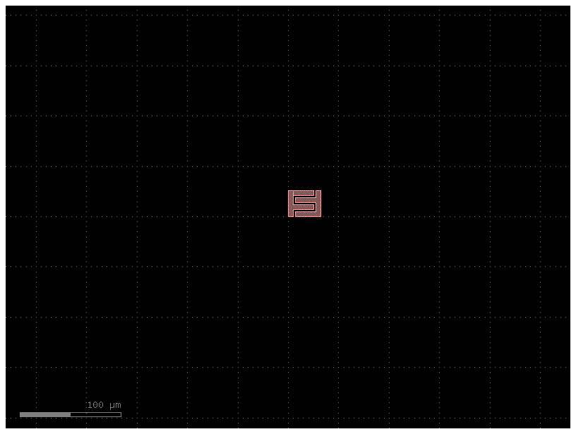
gf.components.interdigital_capacitor draws the two interleaved combs as two disconnected polygons on WG, exposed as the terminals o1 and o2. The enclosing simulation_box on WAFER defines the substrate and vacuum domain passed to the mesher.
simulation_box = [[-200, -200], [200, 200]]
c = gf.Component("capacitance_elmer")
cap = c << gf.components.interdigital_capacitor(
    fingers=4, finger_length=20, finger_gap=2, thickness=5, layer=LAYER.WG
)
c.add_ports(cap.ports)
(xmin, ymin), (xmax, ymax) = simulation_box
c.add_polygon(
    [(xmin, ymin), (xmax, ymin), (xmax, ymax), (xmin, ymax)], layer=LAYER.WAFER
)
c.plot()
Running the simulation
We use the function :func:`~run_capacitive_simulation_elmer`. This runs the simulation and returns an instance of :class:`~ElectrostaticResults` containing the capacitance matrix and a path to the mesh and the field solution.
Help on function run_capacitive_simulation_elmer in module gplugins.elmer.get_capacitance:

run_capacitive_simulation_elmer(component: 'gf.Component', element_order: 'int' = 1, n_processes: 'int' = 1, layer_stack: 'LayerStack | None' = None, material_spec: 'RFMaterialSpec | None' = None, simulation_folder: 'Path | str | None' = None, simulator_params: 'Mapping[str, Any] | None' = None, mesh_parameters: 'dict[str, Any] | None' = None, mesh_file: 'Path | str | None' = None) -> 'ElectrostaticResults'
    Run electrostatic FEM simulations using `Elmer`_.

    Component ports define the capacitor terminals. Conductors touching a port
    are split onto their own layers before meshing so that terminals stay
    disjoint; remaining conductor surfaces are grounded. Returns the field
    solution and Maxwell capacitance matrix.

    .. note:: `ElmerGrid` and `ElmerSolver` must be on PATH. Parallel runs also
        require `ElmerSolver_mpi` and `mpiexec`.

    Args:
        component: Simulation environment as a gdsfactory component.
        element_order: Order of polynomial basis functions.
            Higher is more accurate but takes more memory and time to run.
        n_processes: Number of processes to use for parallelization
        layer_stack: :class:`~LayerStack` defining the simulation layers,
            materials, and thicknesses. A stack with conducting terminals and
            an explicit background volume named by ``background_tag`` is required.
        material_spec:
            :class:`~RFMaterialSpec` defining material parameters for the ones used in ``layer_stack``.
        simulation_folder: Directory for storing the simulation results.
            Default is a temporary directory.
        simulator_params: Elmer-specific parameters. See template file for more details.
        mesh_parameters: Keyword arguments to provide to :func:`meshwell.mesh.mesh`.
            ``background_tag`` names the explicit background volume;
            ``background_padding`` is unsupported by current meshwell.
        mesh_file: Path to a ready mesh to use. Useful for reusing one mesh file.
            By default a mesh is generated according to ``mesh_parameters``.
            The mesh has to contain the terminal surfaces for the component ports.

    .. _Elmer: https://github.com/ElmerCSC/elmerfem
.. note::
   The meshing parameters and element order shown here are very lax. As such, the computed capacitances are not very accurate.
results = run_capacitive_simulation_elmer(
    c,
    layer_stack=layer_stack,
    material_spec=material_spec,
    n_processes=1,
    element_order=1,
    simulation_folder="temporary",
    mesh_parameters=dict(
        background_tag="vacuum",
        default_characteristic_length=200,
        resolution_specs={
            "substrate": [ConstantInField(resolution=40, apply_to="volumes")],
            "vacuum": [ConstantInField(resolution=40, apply_to="volumes")],
            **{
                # `@` separates the layer from the port terminal it belongs to
                f"bw@{port.name}": [ConstantInField(resolution=20, apply_to="volumes")]
                for port in c.ports
            },
        },
    ),
)
assert all(1e-15 < results.capacitance_matrix[port.name, port.name] < 1e-10 for port in c.ports)
print(results.capacitance_matrix)
Info    : Clearing all models and views...
Info    : Done clearing all models and views
Processing ('bw@o1',) - instantiation
Processing ('bw@o2',) - instantiation
Info    : [  0%] Difference
Info : [ 10%] Difference
Info : [ 20%] Difference
Info : [ 30%] Difference - Performing Face-Face intersection
Info : [ 70%] Difference - Projecting edges on faces
Info : [ 80%] Difference - Splitting faces
Info : [ 90%] Difference - Looking for internal shapes
Info : [ 0%] Fragments
Info : [ 10%] Fragments
Info : [ 20%] Fragments
Info : [ 30%] Fragments - Performing Face-Face intersection
Info : [ 70%] Fragments - Projecting edges on faces
Info : [ 80%] Fragments - Splitting faces
Info : [ 90%] Fragments - Checking SD faces
Info : [ 0%] Fragments
Info : [ 10%] Fragments
Info : [ 20%] Fragments
Info : [ 30%] Fragments - Performing Face-Face intersection
Info : [ 70%] Fragments - Projecting edges on faces
Info : [ 80%] Fragments - Splitting faces
Info : [ 90%] Fragments - Checking SD faces
Processing ('substrate',) - instantiation
Info : [ 0%] Difference
Info : [ 10%] Difference
Info : [ 20%] Difference
Info : [ 30%] Difference
Info : [ 40%] Difference
Info : [ 50%] Difference
Info : [ 60%] Difference
Info : [ 70%] Difference
Info : [ 80%] Difference - Making faces
Info : [ 90%] Difference - Looking for internal shapes
Info : [ 0%] Fragments
Info : [ 10%] Fragments
Info : [ 20%] Fragments
Info : [ 30%] Fragments
Info : [ 40%] Fragments
Info : [ 50%] Fragments
Info : [ 60%] Fragments
Info : [ 70%] Fragments - Building splits of containers
Info : [ 80%] Fragments - Splitting faces
Info : [ 90%] Fragments - Checking SD faces
Info : [ 0%] Fragments
Info : [ 10%] Fragments
Info : [ 20%] Fragments
Info : [ 30%] Fragments
Info : [ 40%] Fragments
Info : [ 50%] Fragments
Info : [ 60%] Fragments
Info : [ 70%] Fragments - Building splits of containers
Info : [ 80%] Fragments - Splitting faces
Info : [ 90%] Fragments - Checking SD faces
Processing ('vacuum',) - instantiation
Info : [ 0%] Difference
Info : [ 10%] Difference
Info : [ 20%] Difference
Info : [ 30%] Difference
Info : [ 40%] Difference
Info : [ 50%] Difference
Info : [ 60%] Difference
Info : [ 70%] Difference
Info : [ 80%] Difference - Making faces
Info : [ 90%] Difference - Looking for internal shapes
Info : [ 0%] Fragments
Info : [ 10%] Fragments
Info : [ 20%] Fragments
Info : [ 30%] Fragments
Info : [ 40%] Fragments
Info : [ 50%] Fragments
Info : [ 60%] Fragments
Info : [ 70%] Fragments
Info : [ 80%] Fragments - Splitting faces
Info : [ 90%] Fragments - Filling same domain faces map
Info : [ 0%] Fragments
Info : [ 10%] Fragments
Info : [ 20%] Fragments
Info : [ 30%] Fragments
Info : [ 40%] Fragments
Info : [ 50%] Fragments
Info : [ 60%] Fragments
Info : [ 70%] Fragments - Building splits of containers
Info : [ 80%] Fragments - Splitting faces
Info : [ 90%] Fragments - Checking SD faces
Info : Writing '/home/runner/work/gplugins/gplugins/docs/notebooks/temporary/capacitance_elmer.xao'... Info : Done writing '/home/runner/work/gplugins/gplugins/docs/notebooks/temporary/capacitance_elmer.xao' Info : Clearing all models and views... Info : Done clearing all models and views Info : Reading '/home/runner/work/gplugins/gplugins/docs/notebooks/temporary/capacitance_elmer.xao'... Info : Done reading '/home/runner/work/gplugins/gplugins/docs/notebooks/temporary/capacitance_elmer.xao' Info : Reading '/home/runner/work/gplugins/gplugins/docs/notebooks/temporary/capacitance_elmer.msh'... Info : 171 entities Info : 166 nodes Info : 887 elements Info : Done reading '/home/runner/work/gplugins/gplugins/docs/notebooks/temporary/capacitance_elmer.msh' Info : Writing '/home/runner/work/gplugins/gplugins/docs/notebooks/temporary/capacitance_elmer.msh'... Info : Done writing '/home/runner/work/gplugins/gplugins/docs/notebooks/temporary/capacitance_elmer.msh' ================================================================== ElmerGrid mesh conversion and manipulation utility, Welcome! Version: 26.2 (Rev: NA, Compiled: NA) This program is free software licensed under GPL ================================================================== Elmergrid reading in-line arguments Lower dimensional boundaries will be removed Materials and boundaries will be renumbered Nodes that do not appear in any element will be removed Output will be saved to file capacitance_elmer.
Elmergrid loading data:
-----------------------
Format chosen using the first line: $MeshFormat
Gmsh input file format is type   2.2 in ASCII.
Loading mesh in Gmsh format 2 from file capacitance_elmer.msh
Allocating for 166 knots and 887 elements.
Moving bulk elements to boundary elements
Leading bulk elementtype is 504
Trailing bulk elementtype is 303
There are 328 (out of 887) lower dimensional elements.
Node 160 belongs to maximum of 72 elements
Found 116 side elements that have two parents.
Found correctly 328 side elements.
Parent elements were reordered up to index 559.
Moved 559 elements (out of 887) to new positions
Successfully read the mesh from the Gmsh input file.
Using physical numbering of entities

Elmergrid creating and manipulating meshes:
-------------------------------------------
Removing lower dimensional boundaries
Maximum elementtype is 504 and dimension 3
Minimum elementtype is 504 and dimension 3
Removed 0 (out of 328) less than 2D boundary elements
All 166 nodes were used by the mesh elements
Initial boundary interval [5,13]
BC index changed 5 -> 1 in 8 2D elements of bw_o1___substrate
BC index changed 6 -> 2 in 28 2D elements of bw_o1___vacuum
BC index changed 7 -> 3 in 8 2D elements of bw_o2___substrate
BC index changed 8 -> 4 in 28 2D elements of bw_o2___vacuum
BC index changed 9 -> 5 in 44 2D elements of substrate___vacuum
BC index changed 12 -> 6 in 94 2D elements of substrate___boundary
BC index changed 13 -> 7 in 118 2D elements of vacuum___boundary
Mapping boundary types from [5 13] to [1 7]
Initial body interval [1,4]
Numbering of bodies is already ok
Renumbering of material types completed!
Bounding box of all nodes in mesh:
X:[-200,200] Y:[-200,200] Z:[0,1200]

Notice: the longest bounding box side length of [1200] is greater than 50.
ElmerGUI includes a library of material properties, defined in SI units.  If using ElmerGUI,
then the geometry is expected to have meters as length.  Geometry that exceeds 50 meters
in length or width or height may not be intended.  Many Geometry generators assume
millimeters as the basic unit of length.  Scaling the geometry from millimeters to meters
may be the desired action.  For more help, search the Elmer users forum for posts
about SI units, or for posts about Coordinate Scaling.
Scaling can be accomplished in at least three ways, as follows:
 1. Define the original geometry in meters, not millimeters.
 2. Call ElmerGrid with -scale 0.001 0.001 0.001 as an option.
 3. Add Coordinate Scaling = 0.001 to the simulation section of the sif file.
If using Elmer to analyze large geometry, such as a glacier, then ignore this notice.

Calculate Mesh Pieces in mesh:
There is a single piece in the mesh, so the mesh is conforming.

Elmergrid saving data with method 2:
-------------------------------------
Saving mesh in ElmerSolver format to directory capacitance_elmer.
Saving 166 coordinates to mesh.nodes.
Saving 559 element topologies to mesh.elements.
Saving boundary elements to mesh.boundary.
Saving header info to mesh.header.
Saving names info to mesh.names.
Saving entities info to entities.sif.

Thank you for using ElmerGrid!
Repository: https://github.com/ElmerCSC/elmerfem
Contact: elmeradm@csc.fi
ELMER SOLVER (v 26.2) STARTED AT: 2026/10/20 13:25:19


ParCommInit: Initialize #PEs: 1
MAIN: OMP_NUM_THREADS not set. Using only 1 thread per task.
MAIN:
MAIN: =============================================================
MAIN: ElmerSolver finite element software, Welcome!
MAIN: This program is free software licensed under (L)GPL
MAIN: Copyright April 1st 1995 -> , CSC - IT Center for Science Ltd.
MAIN: Repository https://www.github.org/elmerCSC/elmerfem
MAIN: Homepage https://www.elmerfem.org/,  Email elmeradm@csc.fi
MAIN: Version: 26.2-unknown (Rev: unknown, Compiled: 2026-10-18)
MAIN:  Running one task without MPI parallelization.
MAIN:  Running with just one thread per task.
MAIN:  HYPRE library linked in.
MAIN:  MUMPS library linked in.
MAIN:  Lua interpreter linked in.
MAIN: =============================================================
OpenIncludeFile: Trying to include file: "capacitance_elmer/mesh.names"
MAIN:
MAIN:
MAIN: -------------------------------------
MAIN: Reading Model: /home/runner/work/gplugins/gplugins/docs/notebooks/temporary/capacitance_elmer.sif
LoadInputFile: Scanning input file: /home/runner/work/gplugins/gplugins/docs/notebooks/temporary/capacitance_elmer.sif
LoadInputFile: Scanning only size info
LoadInputFile: First time visiting
LoadInputFile: Reading base load of sif file
OpenIncludeFile: Trying to include file: "capacitance_elmer/mesh.names"
LoadInputFile: Loading input file: /home/runner/work/gplugins/gplugins/docs/notebooks/temporary/capacitance_elmer.sif
LoadInputFile: Reading base load of sif file
OpenIncludeFile: Trying to include file: "capacitance_elmer/mesh.names"
CheckKeyword:  Unlisted keyword: [save all meshes] in section: [solver 2]
LoadInputFile: Number of BCs: 2
LoadInputFile: Number of Body Forces: 0
LoadInputFile: Number of Initial Conditions: 0
LoadInputFile: Number of Materials: 2
LoadInputFile: Number of Equations: 1
LoadInputFile: Number of Solvers: 2
LoadInputFile: Number of Bodies: 4
MAIN:
MAIN: -------------------------------------
MAIN:  Steady state iteration:            1
MAIN: -------------------------------------
MAIN:
   gcr:    10  0.9171E-07  0.9410E-06
ComputeChange: NS (ITER=1) (NRM,RELC): ( 0.55207668      2.0000000     ) :: electrostatics
   gcr:    10  0.7939E-07  0.5988E-06
ComputeChange: NS (ITER=2) (NRM,RELC): ( 0.57114941     0.33960622E-01 ) :: electrostatics
ComputeChange: SS (ITER=1) (NRM,RELC): ( 0.57114941      2.0000000     ) :: electrostatics
MAIN: *** Elmer Solver: ALL DONE ***
MAIN: The end
SOLVER TOTAL TIME(CPU,REAL):         0.06        0.66
ELMER SOLVER FINISHED AT: 2026/10/20 13:25:19
{('o1', 'o1'): 2.541336020248954e-13, ('o1', 'o2'): -2.541336020248964e-13, ('o2', 'o1'): -2.541336020248964e-13, ('o2', 'o2'): 2.541336020248973e-13}
Bibliography
Bibliography
:style: unsrt :filter: docname in docnames