Design a 1x2 MMI
Use Meow's mode solver and EME to find the body width and length of a symmetric 1x2 multimode-interference splitter.
An MMI works by self-imaging: the input field excites many modes of the wide body, and because they travel at different speeds, their interference reproduces the input field as one or more images at specific lengths. For a 1x2 splitter we want the two-fold image to land exactly on the two output tapers.
Component libraries ship default MMI dimensions, but a default may have been chosen for a different stack, wavelength, or taper geometry. Here we start from gdsfactory's default and check it instead of assuming it is right. The workflow is:
- solve the modes of the MMI body and use them to predict where the images should be;
- build a full EME model of the device from its GDS layout;
- map the transmission over a coarse width x length grid;
- refine around the best region;
- check convergence and wavelength response of the chosen design.
import inspect
from itertools import pairwise

import gdsfactory as gf
import matplotlib.pyplot as plt
import numpy as np

import meow as mw

gf.gpdk.PDK.activate()

try:
    import eigenlight  # noqa: F401

    compute_modes = mw.compute_modes_eigenlight
except ModuleNotFoundError:
    # EigenLight is an optional extra (`pip install meow-sim[eigenlight]`).
    compute_modes = mw.compute_modes_tidy3d
print("FDE solver:", compute_modes.__name__)
FDE solver: compute_modes_eigenlight
Meow can use different FDE (mode solver) backends. This notebook uses EigenLight when it is installed and falls back to the Tidy3D solver otherwise. Both return Mode objects, so everything below is independent of that choice.
Quantities to compare
For a unit excitation of the fundamental input mode, define
\(L_\mathrm{ins}\) is the excess loss on top of the ideal 3 dB split. Because the layout is symmetric, \(T_\mathrm{top}\approx T_\mathrm{bottom}\) and the normalized imbalance \(|T_\mathrm{top}-T_\mathrm{bottom}|/T_\mathrm{total}\) is only a sanity check on the port construction. The design objective is to maximize \(T_\mathrm{total}\).
Simulation settings
The taper and waveguide dimensions are fixed; we only design the MMI body. The mesh, number of taper cells, and number of modes are modest so that the notebook runs in a few minutes. We check their effect on the final design at the end.
WAVELENGTH = 1.55
WAVEGUIDE_WIDTH = 0.45
TAPER_WIDTH = 1.0
TAPER_LENGTH = 8.0
GAP_MMI = 0.25  # gap between the two output tapers
NUM_TAPER_CELLS = 12
NUM_MODES = 12
EDGE_OFFSET = 1e-2
GUIDED_INDEX_MIN = 1.45
TE_FRACTION_MIN = 0.5

# gdsfactory's default body size: our starting point, not an assumption.
_defaults = inspect.signature(gf.components.mmi1x2).parameters
DEFAULT_WIDTH_MMI = _defaults["width_mmi"].default
DEFAULT_LENGTH_MMI = _defaults["length_mmi"].default
print(f"gdsfactory default MMI body: {DEFAULT_WIDTH_MMI} um x {DEFAULT_LENGTH_MMI} um")

ENV = mw.Environment(wl=WAVELENGTH, T=25.0)
MESH = mw.Mesh2D(
    x=np.arange(-2.5, 2.5 + 1e-9, 0.05),
    y=np.linspace(-0.75, 0.75, 41),
)
gdsfactory default MMI body: 2.5 um x 5.5 um
Geometry and material extrusion
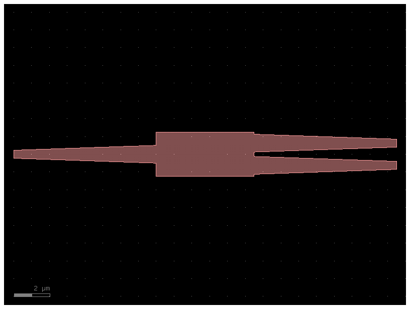
gdsfactory draws the planar 1x2 MMI. Meow uses \(z\) as the propagation direction, so the GDS \(x\) coordinate maps to Meow \(z\), while GDS \(y\) maps to Meow \(x\). The wrapper moves every device to start at \(z=0\).
The oxide cladding extends beyond the simulation window on all sides, so the mode solver's boundaries sit in oxide rather than in air.
def build_mmi(width_mmi: float, length_mmi: float) -> gf.Component:
    mmi = gf.components.mmi1x2(
        width=WAVEGUIDE_WIDTH,
        width_taper=TAPER_WIDTH,
        length_taper=TAPER_LENGTH,
        width_mmi=width_mmi,
        length_mmi=length_mmi,
        gap_mmi=GAP_MMI,
    )
    component = gf.Component()
    reference = component.add_ref(mmi)
    reference.xmin = 0
    return component


def extrusion_rules() -> dict:
    return {
        (1, 0): [
            mw.GdsExtrusionRule(
                material=mw.silicon,
                h_min=0.0,
                h_max=0.22,
                mesh_order=1,
            ),
            mw.GdsExtrusionRule(
                material=mw.silicon_oxide,
                h_min=-2.0,
                h_max=2.0,
                buffer=4.0,
                mesh_order=2,
            ),
        ]
    }


def extrude_mmi(component: gf.Component):
    return mw.extrude_gds(component, extrusion_rules())
EME cells and physical ports
The tapers change width along \(z\), so each is split into several cells. The MMI body has a constant cross-section and needs only one cell. Tiny cells at both ends sample the input and output planes.
Inside the device every cell keeps the full set of computed modes: the tapers and body are where power is exchanged between modes, so the basis should be as complete as practical. The two ends are different: there we want the physical port modes.
- The input port is the fundamental TE mode of the input waveguide.
- At the output plane, the solver returns the symmetric and antisymmetric supermodes of the two output guides. Their order and phase are not port labels. We diagonalize the electric energy contained in the positive-\(x\) half-plane inside that two-mode subspace, which yields one mode localized in each guide, and label them by their power centroids. Positive Meow \(x\) corresponds to the top GDS output.
def make_cells(
    structures, length_mmi: float, *, num_taper_cells=NUM_TAPER_CELLS, mesh=MESH
):
    total_length = 2 * TAPER_LENGTH + length_mmi
    left_edges = np.linspace(0, TAPER_LENGTH, num_taper_cells + 1) + EDGE_OFFSET
    right_edges = (
        np.linspace(TAPER_LENGTH + length_mmi, total_length, num_taper_cells + 1)
        - EDGE_OFFSET
    )
    cell_edges = np.concatenate(
        [left_edges[:1], left_edges, right_edges, right_edges[-1:]]
    )
    return [
        mw.Cell(
            structures=structures, mesh=mesh, z_min=float(z_min), z_max=float(z_max)
        )
        for z_min, z_max in pairwise(cell_edges)
    ]


def guided_te_modes(cross_section, num_modes=NUM_MODES):
    computed = compute_modes(cross_section, num_modes=num_modes)
    guided = [
        mode
        for mode in computed
        if np.real(mode.neff) > GUIDED_INDEX_MIN and mode.te_fraction > TE_FRACTION_MIN
    ]
    if not guided:
        raise RuntimeError("No guided TE modes were found; refine the solver settings.")
    return guided


def combine_modes(modes, coefficients):
    combined = coefficients[0] * modes[0]
    for coefficient, mode in zip(coefficients[1:], modes[1:], strict=True):
        combined = combined + coefficient * mode
    return combined


def mode_power_centroid(mode) -> float:
    density = mw.electric_energy_density(mode)
    x = np.asarray(mode.mesh.Xx)
    return float((x * density).sum() / density.sum())


def localize_output_modes(output_modes):
    if len(output_modes) < 2:
        raise RuntimeError("Two guided TE output supermodes are required.")
    basis = output_modes[:2]
    cross_section = basis[0].cs
    positive_x = np.asarray(basis[0].mesh.Xx) > 0
    eps_x = np.asarray(cross_section.nx) ** 2
    eps_y = np.asarray(cross_section.ny) ** 2
    eps_z = np.asarray(cross_section.nz) ** 2

    # Hermitian energy-overlap operator restricted to the top guide region.
    localization = np.empty((2, 2), dtype=complex)
    for row, mode_a in enumerate(basis):
        for column, mode_b in enumerate(basis):
            cross_density = (
                eps_x * mode_a.Ex.conj() * mode_b.Ex
                + eps_y * mode_a.Ey.conj() * mode_b.Ey
                + eps_z * mode_a.Ez.conj() * mode_b.Ez
            )
            localization[row, column] = cross_density[positive_x].sum()
    localization = 0.5 * (localization + localization.conj().T)

    _, eigenvectors = np.linalg.eigh(localization)
    candidates = [
        combine_modes(basis, eigenvectors[:, -1]),
        combine_modes(basis, eigenvectors[:, 0]),
    ]
    localized = mw.orthonormalize_modes(candidates, mw.inner_product)
    localized.sort(key=mode_power_centroid, reverse=True)
    centroids = [mode_power_centroid(mode) for mode in localized]
    if not (centroids[0] > 0 > centroids[1]):
        message = f"Could not distinguish output guides: {centroids}"
        raise RuntimeError(message)
    return localized


def solve_cell_modes(cells, *, num_modes=NUM_MODES, env=ENV):
    cross_sections = [mw.CrossSection.from_cell(cell=cell, env=env) for cell in cells]
    modes = [compute_modes(cs, num_modes=num_modes) for cs in cross_sections]
    modes[0] = guided_te_modes(cross_sections[0], num_modes)[:1]
    modes[-1] = localize_output_modes(guided_te_modes(cross_sections[-1], num_modes))
    return modes


def transmission_metrics(scattering, port_map) -> dict:
    left = port_map["left@0"]
    top = port_map["right@0"]
    bottom = port_map["right@1"]
    T_top = float(abs(scattering[top, left]) ** 2)
    T_bottom = float(abs(scattering[bottom, left]) ** 2)
    T_total = T_top + T_bottom
    safe_total = max(T_total, 1e-15)
    return {
        "T_top": T_top,
        "T_bottom": T_bottom,
        "T_total": T_total,
        "insertion_loss_db": float(-10 * np.log10(safe_total)),
        "imbalance": abs(T_top - T_bottom) / safe_total,
    }
One complete solve
solve_mmi goes from GDS to S-matrix for one geometry: build, extrude, cut into cells, solve modes in every cell, and cascade the interfaces and propagation sections. We start with gdsfactory's default body size.
def solve_mmi(
    width_mmi: float,
    length_mmi: float,
    *,
    keep_fields: bool = False,
    num_modes: int = NUM_MODES,
    num_taper_cells: int = NUM_TAPER_CELLS,
    mesh: mw.Mesh2D = MESH,
    env: mw.Environment = ENV,
):
    component = build_mmi(width_mmi, length_mmi)
    structures = extrude_mmi(component)
    cells = make_cells(
        structures, length_mmi, num_taper_cells=num_taper_cells, mesh=mesh
    )
    modes = solve_cell_modes(cells, num_modes=num_modes, env=env)
    scattering, port_map = mw.compute_s_matrix(modes, cells=cells)
    result = transmission_metrics(scattering, port_map)
    if keep_fields:
        result.update(
            cells=cells, modes=modes, scattering=scattering, port_map=port_map
        )
    return result
%%time
nominal = solve_mmi(DEFAULT_WIDTH_MMI, DEFAULT_LENGTH_MMI, keep_fields=True)
for name in ("T_top", "T_bottom", "T_total", "insertion_loss_db", "imbalance"):
    print(f"{name:18s}: {nominal[name]:.4f}")
print("modes per cell    :", [len(modes) for modes in nominal["modes"]])
T_top             : 0.4839
T_bottom          : 0.4844
T_total           : 0.9683
insertion_loss_db : 0.1397
imbalance         : 0.0005
modes per cell    : [1, 12, 12, 12, 12, 12, 12, 12, 12, 12, 12, 12, 12, 12, 12, 12, 12, 12, 12, 12, 12, 12, 12, 12, 12, 12, 2]
CPU times: user 41 s, sys: 174 ms, total: 41.2 s
Wall time: 57 s
fig, axes = plt.subplots(1, 3, figsize=(12, 3))
mw.visualize(nominal["modes"][0][0], ax=axes[0], fields=["Ex"], show=False)
mw.visualize(nominal["modes"][-1][0], ax=axes[1], fields=["Ex"], show=False)
mw.visualize(nominal["modes"][-1][1], ax=axes[2], fields=["Ex"], show=False)
axes[0].set_title("Input port")
axes[1].set_title("Top output port")
axes[2].set_title("Bottom output port")
plt.tight_layout()

Predict the image length from the body modes
Before sweeping anything, the modes of the MMI body already tell us where to look. With \(n_0\) and \(n_1\) the effective indices of the two lowest TE body modes, the beat length is
A centered input only excites the symmetric modes, and self-imaging theory then places the two-fold image, which is what a 1x2 splitter needs, at \(L \approx 3L_\pi/8\), and again at \(9L_\pi/8\). In between, at \(3L_\pi/4\), the image is a single spot on the axis, between the two outputs.
body_index = NUM_TAPER_CELLS + 1  # cells: [input, tapers..., body, tapers..., output]
body_modes = [
    mode for mode in nominal["modes"][body_index] if mode.te_fraction > TE_FRACTION_MIN
]
body_neffs = np.array([float(np.real(mode.neff)) for mode in body_modes])
print("TE body mode indices:", np.round(body_neffs, 4))

x = np.asarray(body_modes[0].mesh.Xx)[:, 0]
y_core = np.argmax(np.abs(np.asarray(body_modes[0].Ex)).max(axis=0))
plt.figure(figsize=(8, 3))
for mode in body_modes[:5]:
    profile = np.real(np.asarray(mode.Ex)[:, y_core])
    profile = profile / profile[np.argmax(np.abs(profile))]
    plt.plot(x, profile, label=f"n_eff = {float(np.real(mode.neff)):.4f}")
plt.axvspan(-DEFAULT_WIDTH_MMI / 2, DEFAULT_WIDTH_MMI / 2, color="0.9", zorder=-1)
plt.xlabel("x [um]")
plt.ylabel("Ex (normalized)")
plt.title("Lowest TE modes of the MMI body")
plt.legend(fontsize=7, loc="lower right")
plt.tight_layout()


def beat_length(body_modes, wavelength=WAVELENGTH) -> float:
    te = sorted(
        (
            float(np.real(mode.neff))
            for mode in body_modes
            if mode.te_fraction > TE_FRACTION_MIN
        ),
        reverse=True,
    )
    return wavelength / (2 * (te[0] - te[1]))


L_pi = beat_length(body_modes)
print(
    f"L_pi = {L_pi:.2f} um -> first two-fold image near 3 L_pi / 8 = {3 * L_pi / 8:.2f} um"
)
TE body mode indices: [2.8241 2.7738 2.6882 2.5645 2.398  2.1817 1.906  1.5787]
L_pi = 15.40 um -> first two-fold image near 3 L_pi / 8 = 5.77 um
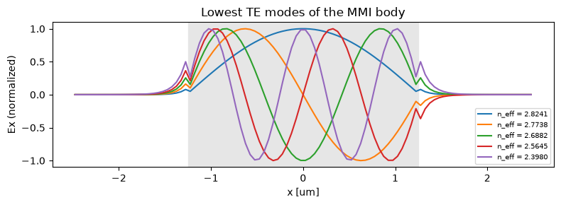
This is only an estimate: the tapers are wide and close together, and the self-imaging formula assumes a quadratic mode spectrum. EME does not make that assumption, so we use the prediction to choose the sweep range and let the full simulation decide.
Coarse sweep over width and length
A full solve takes several seconds, most of it spent solving modes in the taper cells. For this sweep, it pays to ask which parts of the EME model actually change:
- Body width. The taper cross-sections do not depend on the body at all, so their modes stay the same. For a new width we build the GDS again, but only the body cross-section needs new modes, followed by new interface S-matrices.
- Body length. Nothing changes in any cross-section. Only the propagation distance of the body cell changes, so each length only needs a new cascade.
Both shortcuts are exact for this device. If you sweep a parameter that changes the tapers, such as TAPER_WIDTH, go back to solve_mmi. We check the shortcut against a full solve at the end.
def solve_width(width_mmi: float, reference=nominal):
    component = build_mmi(width_mmi, DEFAULT_LENGTH_MMI)
    body_cell = make_cells(extrude_mmi(component), DEFAULT_LENGTH_MMI)[body_index]
    body_cross_section = mw.CrossSection.from_cell(cell=body_cell, env=ENV)
    modes = list(reference["modes"])  # taper and port modes do not depend on the body
    modes[body_index] = compute_modes(body_cross_section, num_modes=NUM_MODES)
    return {
        "cell_lengths": [cell.z_max - cell.z_min for cell in reference["cells"]],
        "modes": modes,
        "interfaces": mw.compute_interface_s_matrices(modes),
        "L_pi": beat_length(modes[body_index]),
    }


def metrics_at_length(solution, length_mmi: float) -> dict:
    cell_lengths = list(solution["cell_lengths"])
    cell_lengths[body_index] = length_mmi - 2 * EDGE_OFFSET
    scattering, port_map = mw.compute_s_matrix(
        solution["modes"],
        cell_lengths=cell_lengths,
        interfaces_fn=lambda _modes: solution["interfaces"],
    )
    return transmission_metrics(scattering, port_map)


metric_names = ("T_top", "T_bottom", "T_total", "insertion_loss_db", "imbalance")


def sweep(widths_mmi, lengths_mmi):
    shape = (len(widths_mmi), len(lengths_mmi))
    metrics = {name: np.zeros(shape) for name in metric_names}
    beat_lengths = np.zeros(len(widths_mmi))
    for width_index, width_mmi in enumerate(widths_mmi):
        solution = solve_width(float(width_mmi))
        beat_lengths[width_index] = solution["L_pi"]
        for length_index, length_mmi in enumerate(lengths_mmi):
            result = metrics_at_length(solution, float(length_mmi))
            for name in metric_names:
                metrics[name][width_index, length_index] = result[name]
        best = np.argmax(metrics["T_total"][width_index])
        print(
            f"width={width_mmi:.3f} um: L_pi={solution['L_pi']:5.2f} um, "
            f"best length={lengths_mmi[best]:.2f} um, "
            f"T_total={metrics['T_total'][width_index, best]:.4f}"
        )
    return metrics, beat_lengths
%%time
widths_mmi = np.round(np.arange(2.0, 3.01, 0.1), 3)
lengths_mmi = np.round(np.arange(2.0, 20.01, 0.5), 3)
coarse, coarse_L_pi = sweep(widths_mmi, lengths_mmi)
width=2.000 um: L_pi= 9.84 um, best length=18.00 um, T_total=0.8945


width=2.100 um: L_pi=10.85 um, best length=20.00 um, T_total=0.9144


width=2.200 um: L_pi=11.92 um, best length=4.50 um, T_total=0.9335


width=2.300 um: L_pi=13.03 um, best length=4.50 um, T_total=0.9513


width=2.400 um: L_pi=14.19 um, best length=5.00 um, T_total=0.9663


width=2.500 um: L_pi=15.40 um, best length=5.50 um, T_total=0.9683


width=2.600 um: L_pi=16.66 um, best length=6.00 um, T_total=0.9604


width=2.700 um: L_pi=17.96 um, best length=6.50 um, T_total=0.9448


width=2.800 um: L_pi=19.32 um, best length=7.00 um, T_total=0.9227


width=2.900 um: L_pi=20.72 um, best length=7.50 um, T_total=0.8942


width=3.000 um: L_pi=22.18 um, best length=8.00 um, T_total=0.8582
CPU times: user 1min 37s, sys: 7.58 s, total: 1min 45s
Wall time: 1min 35s
def plot_map(ax, widths, lengths, values, title, label, cmap="viridis", **kwargs):
    image = ax.pcolormesh(
        lengths, widths, values, shading="nearest", cmap=cmap, **kwargs
    )
    ax.set_xlabel("MMI length [um]")
    ax.set_ylabel("MMI width [um]")
    ax.set_title(title)
    plt.colorbar(image, ax=ax, label=label)


fig, ax = plt.subplots(figsize=(10, 4))
plot_map(
    ax, widths_mmi, lengths_mmi, coarse["T_total"], "Total transmission", "T_total"
)
for factor, style, label in (
    (3 / 8, "-", "3 L_pi / 8"),
    (3 / 4, ":", "3 L_pi / 4"),
    (9 / 8, "--", "9 L_pi / 8"),
):
    ax.plot(factor * coarse_L_pi, widths_mmi, "w" + style, lw=1.5, label=label)
ax.set_xlim(lengths_mmi[0], lengths_mmi[-1])
ax.legend(loc="upper right", fontsize=8)
plt.tight_layout()

width_index, length_index = np.unravel_index(
    np.argmax(coarse["T_total"]), coarse["T_total"].shape
)
coarse_best = (float(widths_mmi[width_index]), float(lengths_mmi[length_index]))
print(
    f"coarse optimum: width={coarse_best[0]:.2f} um, length={coarse_best[1]:.2f} um, "
    f"T_total={coarse['T_total'][width_index, length_index]:.4f}"
)
coarse optimum: width=2.50 um, length=5.50 um, T_total=0.9683
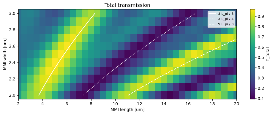
The map shows the self-imaging pattern. The bright ridge follows the two-fold image at \(3L_\pi/8\) and moves to longer lengths as the body gets wider, since \(L_\pi \propto W^2\). Along \(3L_\pi/4\) the image collapses to a single spot on the axis and little light reaches the outputs. A second bright ridge appears near \(9L_\pi/8\). It also splits the light, but it is roughly three times longer and more sensitive to width and wavelength, so we design on the first ridge.
The width matters as well as the length. The two images sit roughly a quarter of the body width either side of the axis, while the output tapers sit at a fixed ±(GAP_MMI + TAPER_WIDTH)/2. The ridge is brightest at the width where the two coincide.
Refine around the best region
Now zoom in with a finer grid around the coarse optimum.
%%time
# gdsfactory snaps port widths to a 2 nm grid, so keep width steps even in nm.
fine_widths = np.round(coarse_best[0] + np.arange(-0.1, 0.1001, 0.02), 3)
fine_lengths = np.round(coarse_best[1] + np.arange(-0.75, 0.7501, 0.05), 3)
fine, fine_L_pi = sweep(fine_widths, fine_lengths)
width=2.400 um: L_pi=14.19 um, best length=5.05 um, T_total=0.9668


width=2.420 um: L_pi=14.41 um, best length=5.20 um, T_total=0.9675


width=2.440 um: L_pi=14.65 um, best length=5.25 um, T_total=0.9686


width=2.460 um: L_pi=14.85 um, best length=5.30 um, T_total=0.9687


width=2.480 um: L_pi=15.05 um, best length=5.35 um, T_total=0.9682


width=2.500 um: L_pi=15.40 um, best length=5.50 um, T_total=0.9683


width=2.520 um: L_pi=15.62 um, best length=5.55 um, T_total=0.9676


width=2.540 um: L_pi=15.88 um, best length=5.65 um, T_total=0.9657


width=2.560 um: L_pi=16.09 um, best length=5.75 um, T_total=0.9652


width=2.580 um: L_pi=16.29 um, best length=5.80 um, T_total=0.9642


width=2.600 um: L_pi=16.66 um, best length=5.95 um, T_total=0.9605
CPU times: user 1min 23s, sys: 6.38 s, total: 1min 29s
Wall time: 1min 21s
fig, axes = plt.subplots(1, 2, figsize=(13, 3.8))
plot_map(
    axes[0],
    fine_widths,
    fine_lengths,
    fine["T_total"],
    "Total transmission (refined)",
    "T_total",
)
plot_map(
    axes[1],
    fine_widths,
    fine_lengths,
    fine["insertion_loss_db"],
    "Excess loss (refined)",
    "dB",
    cmap="magma_r",
)
width_index, length_index = np.unravel_index(
    np.argmax(fine["T_total"]), fine["T_total"].shape
)
best_width = float(fine_widths[width_index])
best_length = float(fine_lengths[length_index])
for ax in axes:
    ax.plot(best_length, best_width, "c*", ms=12)
plt.tight_layout()
print(f"refined optimum: width={best_width:.3f} um, length={best_length:.2f} um")
if best_width in (fine_widths[0], fine_widths[-1]) or best_length in (
    fine_lengths[0],
    fine_lengths[-1],
):
    print(
        "The optimum is on the edge of the refined grid: move or enlarge the grid and rerun."
    )
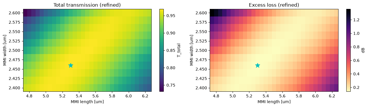
refined optimum: width=2.460 um, length=5.30 um
fig, axes = plt.subplots(1, 2, figsize=(12, 3.2))
for width_index_ in range(0, len(fine_widths), 2):
    axes[0].plot(
        fine_lengths,
        fine["T_total"][width_index_],
        label=f"W={fine_widths[width_index_]:.3f}",
    )
axes[0].set_xlabel("MMI length [um]")
axes[0].set_ylabel("T_total")
axes[0].legend(fontsize=7)
axes[0].grid(alpha=0.3)
axes[1].plot(fine_widths, fine["T_total"][:, length_index], "o-")
axes[1].set_xlabel("MMI width [um]")
axes[1].set_title(f"length = {best_length:.2f} um")
axes[1].grid(alpha=0.3)
plt.tight_layout()
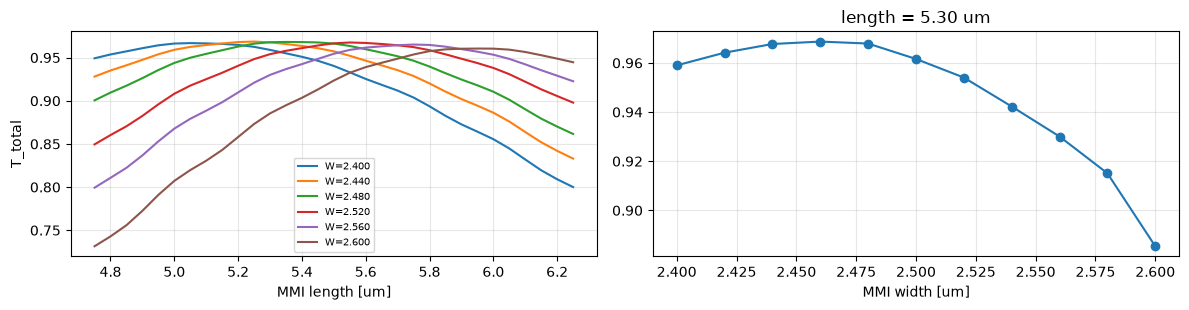
The high-transmission region is a diagonal ridge: a wider body needs a longer body, because \(L_\pi \propto W^2\). Along the ridge the transmission is almost constant, so there is a whole family of nearly equivalent designs. Away from it, the transmission drops quickly. The right-hand slice shows the width tolerance at the chosen length, which is the number to compare with your fabrication process.
Check the chosen design
First we re-solve the chosen geometry from scratch with solve_mmi. This confirms that the shortcuts used in the sweep agree with a direct simulation. We compare it with the gdsfactory default we started from.
best = solve_mmi(best_width, best_length, keep_fields=True)
start = nominal
print(f"{'':28s}{'T_top':>8s}{'T_bottom':>10s}{'T_total':>9s}{'loss [dB]':>11s}")
for label, result in (
    (f"default W={DEFAULT_WIDTH_MMI:.3f} L={DEFAULT_LENGTH_MMI:5.2f}", start),
    (f"design  W={best_width:.3f} L={best_length:5.2f}", best),
):
    print(
        f"{label:28s}{result['T_top']:8.4f}{result['T_bottom']:10.4f}"
        f"{result['T_total']:9.4f}{result['insertion_loss_db']:11.3f}"
    )
print(
    f"sweep value at the design point: T_total={fine['T_total'][width_index, length_index]:.4f}"
)
                               T_top  T_bottom  T_total  loss [dB]
default W=2.500 L= 5.50       0.4839    0.4844   0.9683      0.140
design  W=2.460 L= 5.30       0.4841    0.4846   0.9687      0.138
sweep value at the design point: T_total=0.9687
The full solve reproduces the sweep value, so the shortcuts were exact. The refined optimum and gdsfactory's default differ by much less than the numerical uncertainty estimated below. For this stack, wavelength, and taper, the default already lies on the optimum ridge. We learned that from the sweep rather than assuming it. Change any of those and the ridge moves, so the workflow, not the number, is what carries over.
z = np.linspace(best["cells"][0].z_min, best["cells"][-1].z_max, 400)
field, x = mw.propagate_modes(best["modes"], best["cells"], z=z, y=0.11)
plt.figure(figsize=(10, 3))
plt.pcolormesh(z, x, np.abs(field).T, shading="auto", cmap="magma")
plt.axvline(TAPER_LENGTH, color="w", lw=0.5)
plt.axvline(TAPER_LENGTH + best_length, color="w", lw=0.5)
plt.xlabel("z [um]")
plt.ylabel("x [um]")
plt.title(f"|Ex| in the designed MMI (W={best_width:.3f} um, L={best_length:.2f} um)")
plt.colorbar(label="|Ex|")
plt.tight_layout()
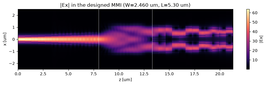
The input is imaged onto the two output tapers at the end of the body. The small steps visible in the tapers come from the staircase approximation: inside each cell the field is rebuilt from that cell's own modes.
Convergence
A design is only as good as the simulation behind it. We re-solve the chosen geometry with more modes, more taper cells, and a finer mesh, one setting at a time. If \(T_\mathrm{total}\) changes by more than you can tolerate, increase that setting and repeat the sweep.
The taper discretization deserves special attention. EME approximates each taper by a staircase, and every step scatters a little power into modes that do not reach the outputs. With too few cells this loss is large enough to distort the sweep, so the row with 6 taper cells shows what an under-resolved model looks like.
%%time
fine_mesh = mw.Mesh2D(
    x=np.arange(-2.5, 2.5 + 1e-9, 0.035), y=np.linspace(-0.75, 0.75, 61)
)
variations = {
    "6 taper cells": {"num_taper_cells": 6},
    "baseline": {},
    "num_modes = 20": {"num_modes": 20},
    "24 taper cells": {"num_taper_cells": 24},
    "finer mesh": {"mesh": fine_mesh},
}
for label, overrides in variations.items():
    result = solve_mmi(best_width, best_length, **overrides)
    print(
        f"{label:16s}: T_total={result['T_total']:.4f}  loss={result['insertion_loss_db']:.3f} dB"
    )
6 taper cells   : T_total=0.9127  loss=0.397 dB


baseline        : T_total=0.9687  loss=0.138 dB


num_modes = 20  : T_total=0.9663  loss=0.149 dB


24 taper cells  : T_total=0.9716  loss=0.125 dB


finer mesh      : T_total=0.9697  loss=0.134 dB
CPU times: user 2min 59s, sys: 1.03 s, total: 3min
Wall time: 2min 58s
Wavelength response
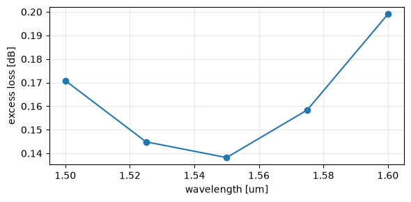
Finally, re-solve the chosen design at a few wavelengths. Every wavelength changes the material indices and the mode solutions, so each point is a full solve. Because \(L_\pi\) scales roughly as \(1/\lambda\), the image moves slowly with wavelength, and a short MMI like this one is broadband.
%%time
wavelengths = np.linspace(1.50, 1.60, 5)
spectrum = [
    best
    if np.isclose(wl, WAVELENGTH)
    else solve_mmi(best_width, best_length, env=mw.Environment(wl=float(wl), T=25.0))
    for wl in wavelengths
]
plt.figure(figsize=(6, 3))
plt.plot(wavelengths, [r["insertion_loss_db"] for r in spectrum], "o-")
plt.xlabel("wavelength [um]")
plt.ylabel("excess loss [dB]")
plt.grid(alpha=0.3)
plt.tight_layout()
CPU times: user 1min 56s, sys: 434 ms, total: 1min 56s
Wall time: 1min 56s
Next steps
- The taper width, taper length, and output gap were held fixed. They set how well the images couple into the outputs, so they are natural next design variables. Add them as outer loops around
sweep, with a full rebuild for each value. - Before fabrication, repeat the convergence study with tighter settings and a wider simulation window, and check tolerance to width, thickness, and etch variations.