

Models#
airbridge#
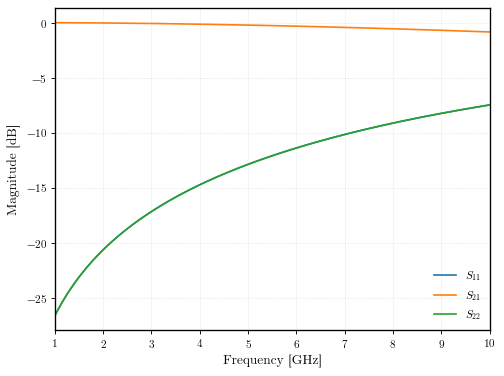
- qpdk.models.airbridge(f=5000000000.0, cpw_width=10.0, bridge_width=10.0, airgap_height=3.0, loss_tangent=1.2e-08)[source]#
S-parameter model for a superconducting CPW airbridge.
The airbridge is modeled as a lumped lossy shunt admittance (accounting for dielectric loss and shunt capacitance) embedded between two sections of transmission line that represent the physical footprint of the bridge.
Parallel plate capacitor model is as done in [CMK+14] The default value for the loss tangent \(\tan\,\delta\) is also taken from there.
- Parameters:
f (Annotated[Array | ndarray | Annotated[Annotated[int | integer, PlainValidator(func=~sax.saxtypes.core.val_int, json_schema_input_type=~typing.Any)] | float | floating, PlainValidator(func=~sax.saxtypes.core.val_float, json_schema_input_type=~typing.Any)], floating, PlainValidator(func=~sax.saxtypes.core.val_float_array, json_schema_input_type=~typing.Any)]) – Array of frequency points in Hz
cpw_width (Annotated[float | floating, PlainValidator(func=~sax.saxtypes.core.val_float, json_schema_input_type=~typing.Any)]) – Width of the CPW center conductor in µm.
bridge_width (Annotated[float | floating, PlainValidator(func=~sax.saxtypes.core.val_float, json_schema_input_type=~typing.Any)]) – Width of the airbridge in µm.
airgap_height (Annotated[float | floating, PlainValidator(func=~sax.saxtypes.core.val_float, json_schema_input_type=~typing.Any)]) – Height of the airgap in µm.
loss_tangent (Annotated[float | floating, PlainValidator(func=~sax.saxtypes.core.val_float, json_schema_input_type=~typing.Any)]) – Dielectric loss tangent of the supporting layer/residues.
- Returns:
S-parameters dictionary
- Return type:
sax.SDict
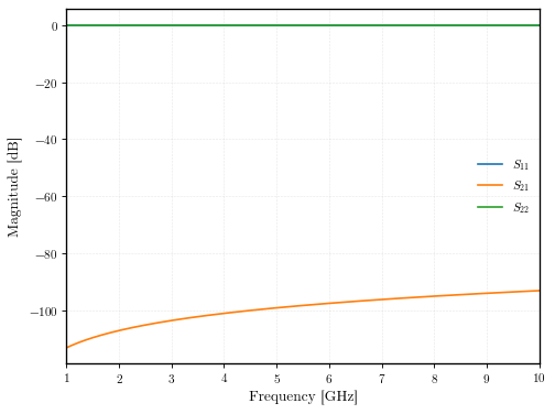
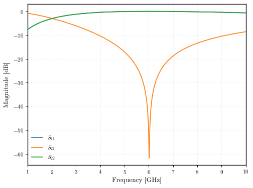
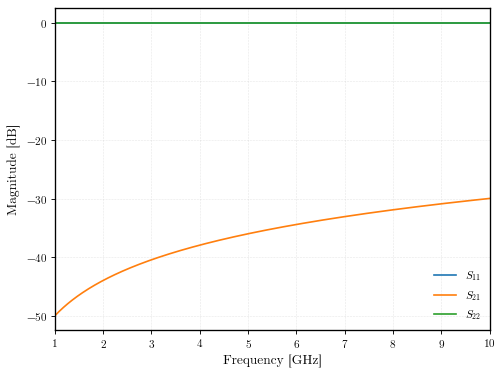
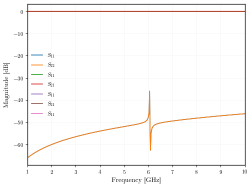
(Source code, svg, pdf, png)

qpdk.models.airbridge() S-parameters for \(f\in[1,10]\,\mathrm{GHz}\).#
bend_circular#
- qpdk.models.bend_circular(f=5000000000.0, length=1000, cross_section='cpw')[source]#
S-parameter model for a circular bend, wrapped to
straight().- Parameters:
f (Annotated[Array | ndarray | Annotated[Annotated[int | integer, PlainValidator(func=~sax.saxtypes.core.val_int, json_schema_input_type=~typing.Any)] | float | floating, PlainValidator(func=~sax.saxtypes.core.val_float, json_schema_input_type=~typing.Any)], floating, PlainValidator(func=~sax.saxtypes.core.val_float_array, json_schema_input_type=~typing.Any)]) – Array of frequency points in Hz
length (Annotated[float | floating, PlainValidator(func=~sax.saxtypes.core.val_float, json_schema_input_type=~typing.Any)]) – Physical length in µm
cross_section (CrossSectionSpec) – The cross-section of the waveguide.
- Returns:
S-parameters dictionary
- Return type:
sax.SDict
(Source code, svg, pdf, png)

qpdk.models.bend_circular() S-parameters for \(f\in[1,10]\,\mathrm{GHz}\).#
bend_circular_all_angle#
- qpdk.models.bend_circular_all_angle(f=5000000000.0, length=1000, cross_section='cpw')[source]#
S-parameter model for a circular bend, wrapped to
straight().- Parameters:
f (Annotated[Array | ndarray | Annotated[Annotated[int | integer, PlainValidator(func=~sax.saxtypes.core.val_int, json_schema_input_type=~typing.Any)] | float | floating, PlainValidator(func=~sax.saxtypes.core.val_float, json_schema_input_type=~typing.Any)], floating, PlainValidator(func=~sax.saxtypes.core.val_float_array, json_schema_input_type=~typing.Any)]) – Array of frequency points in Hz
length (Annotated[float | floating, PlainValidator(func=~sax.saxtypes.core.val_float, json_schema_input_type=~typing.Any)]) – Physical length in µm
cross_section (CrossSectionSpec) – The cross-section of the waveguide.
- Returns:
S-parameters dictionary
- Return type:
sax.SDict
(Source code, svg, pdf, png)

qpdk.models.bend_circular_all_angle() S-parameters for \(f\in[1,10]\,\mathrm{GHz}\).#
bend_euler#
- qpdk.models.bend_euler(f=5000000000.0, length=1000, cross_section='cpw')[source]#
S-parameter model for an Euler bend, wrapped to
straight().- Parameters:
f (Annotated[Array | ndarray | Annotated[Annotated[int | integer, PlainValidator(func=~sax.saxtypes.core.val_int, json_schema_input_type=~typing.Any)] | float | floating, PlainValidator(func=~sax.saxtypes.core.val_float, json_schema_input_type=~typing.Any)], floating, PlainValidator(func=~sax.saxtypes.core.val_float_array, json_schema_input_type=~typing.Any)]) – Array of frequency points in Hz
length (Annotated[float | floating, PlainValidator(func=~sax.saxtypes.core.val_float, json_schema_input_type=~typing.Any)]) – Physical length in µm
cross_section (CrossSectionSpec) – The cross-section of the waveguide.
- Returns:
S-parameters dictionary
- Return type:
sax.SDict
(Source code, svg, pdf, png)

qpdk.models.bend_euler() S-parameters for \(f\in[1,10]\,\mathrm{GHz}\).#
bend_euler_all_angle#
- qpdk.models.bend_euler_all_angle(f=5000000000.0, length=1000, cross_section='cpw')[source]#
S-parameter model for an Euler bend, wrapped to
straight().- Parameters:
f (Annotated[Array | ndarray | Annotated[Annotated[int | integer, PlainValidator(func=~sax.saxtypes.core.val_int, json_schema_input_type=~typing.Any)] | float | floating, PlainValidator(func=~sax.saxtypes.core.val_float, json_schema_input_type=~typing.Any)], floating, PlainValidator(func=~sax.saxtypes.core.val_float_array, json_schema_input_type=~typing.Any)]) – Array of frequency points in Hz
length (Annotated[float | floating, PlainValidator(func=~sax.saxtypes.core.val_float, json_schema_input_type=~typing.Any)]) – Physical length in µm
cross_section (CrossSectionSpec) – The cross-section of the waveguide.
- Returns:
S-parameters dictionary
- Return type:
sax.SDict
(Source code, svg, pdf, png)

qpdk.models.bend_euler_all_angle() S-parameters for \(f\in[1,10]\,\mathrm{GHz}\).#
bend_s#
- qpdk.models.bend_s(f=5000000000.0, length=1000, cross_section='cpw')[source]#
S-parameter model for an S-bend, wrapped to
straight().- Parameters:
f (Annotated[Array | ndarray | Annotated[Annotated[int | integer, PlainValidator(func=~sax.saxtypes.core.val_int, json_schema_input_type=~typing.Any)] | float | floating, PlainValidator(func=~sax.saxtypes.core.val_float, json_schema_input_type=~typing.Any)], floating, PlainValidator(func=~sax.saxtypes.core.val_float_array, json_schema_input_type=~typing.Any)]) – Array of frequency points in Hz
length (Annotated[float | floating, PlainValidator(func=~sax.saxtypes.core.val_float, json_schema_input_type=~typing.Any)]) – Physical length in µm
cross_section (CrossSectionSpec) – The cross-section of the waveguide.
- Returns:
S-parameters dictionary
- Return type:
sax.SDict
(Source code, svg, pdf, png)

qpdk.models.bend_s() S-parameters for \(f\in[1,10]\,\mathrm{GHz}\).#
coupler_ring#
- qpdk.models.coupler_ring(f=5000000000.0, length=20.0, gap=0.27, cross_section='cpw')[source]#
S-parameter model for two coupled coplanar waveguides in a ring configuration.
The implementation is the same as straight coupler for now.
TODO: Fetch coupling capacitance from a curved simulation library.
- Parameters:
f (Array | ndarray | bool | number | bool | int | float | complex | TypedNdArray) – Array of frequency points in Hz
length (int | float) – Physical length of coupling section in µm
gap (int | float) – Gap between the coupled waveguides in µm
cross_section (CrossSectionSpec) – The cross-section of the CPW.
- Returns:
S-parameters dictionary
- Return type:
sax.SDict
(Source code, svg, pdf, png)

qpdk.models.coupler_ring() S-parameters for \(f\in[1,10]\,\mathrm{GHz}\).#
coupler_straight#
- qpdk.models.coupler_straight(f=5000000000.0, length=20.0, gap=0.27, cross_section='cpw')[source]#
S-parameter model for two coupled coplanar waveguides,
coupler_straight().- Parameters:
f (Array | ndarray | bool | number | bool | int | float | complex | TypedNdArray) – Array of frequency points in Hz
length (int | float) – Physical length of coupling section in µm
gap (int | float) – Gap between the coupled waveguides in µm
cross_section (CrossSectionSpec) – The cross-section of the CPW.
- Returns:
S-parameters dictionary
- Return type:
sax.SDict
o2──────▲───────o3
        │gap
o1──────▼───────o4
(Source code, svg, pdf, png)

qpdk.models.coupler_straight() S-parameters for \(f\in[1,10]\,\mathrm{GHz}\).#
coupling_strength_to_capacitance#
- qpdk.models.coupling_strength_to_capacitance(g_ghz, c_sigma, c_r, f_q_ghz, f_r_ghz)[source]#
Convert coupling strength \(g\) to coupling capacitance \(C_c\).
In the dispersive limit (\(g \ll f_q, f_r\)), the coupling strength can be related to a coupling capacitance via:
\[g \approx \frac{1}{2} \frac{C_c}{\sqrt{C_\Sigma C_r}} \sqrt{f_q f_r}\]Solving for \(C_c\):
\[C_c = \frac{2g}{\sqrt{f_q f_r}} \sqrt{C_\Sigma C_r}\]See [KKY+19, Sav23] for details.
- Parameters:
- Returns:
Coupling capacitance in Farads.
- Return type:
Example
>>> C_c = coupling_strength_to_capacitance(
...     g_ghz=0.1,
...     c_sigma=100e-15,  # 100 fF
...     c_r=50e-15,  # 50 fF
...     f_q_ghz=5.0,
...     f_r_ghz=7.0,
... )
>>> print(f"{C_c * 1e15:.2f} fF")
cpw_cpw_coupling_capacitance#
- qpdk.models.cpw_cpw_coupling_capacitance(f, length, gap, cross_section)[source]#
Calculate the coupling capacitance between two parallel CPWs.
- Parameters:
f (Annotated[Array | ndarray | Annotated[Annotated[int | integer, PlainValidator(func=~sax.saxtypes.core.val_int, json_schema_input_type=~typing.Any)] | float | floating, PlainValidator(func=~sax.saxtypes.core.val_float, json_schema_input_type=~typing.Any)], floating, PlainValidator(func=~sax.saxtypes.core.val_float_array, json_schema_input_type=~typing.Any)]) – Frequency array in Hz.
length (float | Array | ndarray | bool | number | bool | int | complex | TypedNdArray) – The coupling length in µm.
gap (float | Array | ndarray | bool | number | bool | int | complex | TypedNdArray) – The gap between the two center conductors in µm.
cross_section (CrossSectionSpec) – The cross-section of the CPW.
- Returns:
The total coupling capacitance in Farads.
- Return type:
cpw_epsilon_eff#
- qpdk.models.cpw_epsilon_eff(w, s, h, ep_r)[source]#
Effective permittivity of a CPW on a finite-height substrate.
\[\begin{split}\begin{aligned} k_0 &= \frac{w}{w + 2s} \\ k_1 &= \frac{\sinh(\pi w / 4h)}{\sinh\bigl(\pi(w + 2s) / 4h\bigr)} \\ q_1 &= \frac{K(k_1^2)/K(1 - k_1^2)}{K(k_0^2)/K(1 - k_0^2)} \\ \varepsilon_{\mathrm{eff}} &= 1 + \frac{q_1(\varepsilon_r - 1)}{2} \end{aligned}\end{split}\]where \(K\) is the complete elliptic integral of the first kind in the parameter convention (\(m = k^2\)).
References
Simoons, Eq. 2.37; Ghione & Naldi
- Parameters:
w (Annotated[Array | ndarray | Annotated[Annotated[int | integer, PlainValidator(func=~sax.saxtypes.core.val_int, json_schema_input_type=~typing.Any)] | float | floating, PlainValidator(func=~sax.saxtypes.core.val_float, json_schema_input_type=~typing.Any)], floating, PlainValidator(func=~sax.saxtypes.core.val_float_array, json_schema_input_type=~typing.Any)]) – Centre-conductor width (m).
s (Annotated[Array | ndarray | Annotated[Annotated[int | integer, PlainValidator(func=~sax.saxtypes.core.val_int, json_schema_input_type=~typing.Any)] | float | floating, PlainValidator(func=~sax.saxtypes.core.val_float, json_schema_input_type=~typing.Any)], floating, PlainValidator(func=~sax.saxtypes.core.val_float_array, json_schema_input_type=~typing.Any)]) – Gap to ground plane (m).
h (Annotated[Array | ndarray | Annotated[Annotated[int | integer, PlainValidator(func=~sax.saxtypes.core.val_int, json_schema_input_type=~typing.Any)] | float | floating, PlainValidator(func=~sax.saxtypes.core.val_float, json_schema_input_type=~typing.Any)], floating, PlainValidator(func=~sax.saxtypes.core.val_float_array, json_schema_input_type=~typing.Any)]) – Substrate height (m).
ep_r (Annotated[Array | ndarray | Annotated[Annotated[int | integer, PlainValidator(func=~sax.saxtypes.core.val_int, json_schema_input_type=~typing.Any)] | float | floating, PlainValidator(func=~sax.saxtypes.core.val_float, json_schema_input_type=~typing.Any)], floating, PlainValidator(func=~sax.saxtypes.core.val_float_array, json_schema_input_type=~typing.Any)]) – Relative permittivity of the substrate.
- Returns:
Effective permittivity (dimensionless).
- Return type:
cpw_parameters#
- qpdk.models.cpw_parameters(width, gap, *, tand=None)[source]#
Compute complex effective permittivity and characteristic impedance for a CPW.
Uses the JAX-jittable functions from
sax.models.rfwith the PDK layer stack (substrate height, conductor thickness, material permittivity).Dielectric loss is included via the filling factor \(q\) and the provided tand:
\[\varepsilon_{\text{eff, complex}} = \varepsilon_{\text{eff}} \left( 1 - j q \frac{\varepsilon_r}{\varepsilon_{\text{eff}}} \tan \delta \right)\]where \(q = (\varepsilon_{\text{eff}} - 1) / (\varepsilon_r - 1)\).
Conductor thickness corrections follow Gupta, Garg, Bahl & Bhartia [GGBB96] (§7.3, Eqs. 7.98-7.100).
- Parameters:
- Returns:
(ep_eff, z0)— complex effective permittivity (dimensionless) and characteristic impedance (Ω).- Return type:
cpw_thickness_correction#
- qpdk.models.cpw_thickness_correction(w, s, t, ep_eff)[source]#
Apply conductor thickness correction to CPW ε_eff and Z₀.
First-order correction from Gupta, Garg, Bahl & Bhartia
\[\begin{split}\begin{aligned} \Delta &= \frac{1.25\,t}{\pi} \left(1 + \ln\\frac{4\pi w}{t}\right) \\ k_e &= k_0 + (1 - k_0^2)\,\frac{\Delta}{2s} \\ \varepsilon_{\mathrm{eff},t} &= \varepsilon_{\mathrm{eff}} - \frac{0.7\,(\varepsilon_{\mathrm{eff}} - 1)\,t/s} {K(k_0^2)/K(1-k_0^2) + 0.7\,t/s} \\ Z_{0,t} &= \frac{30\pi} {\sqrt{\varepsilon_{\mathrm{eff},t}}\; K(k_e^2)/K(1-k_e^2)} \end{aligned}\end{split}\]References
Gupta, Garg, Bahl & Bhartia, §7.3, Eqs. 7.98-7.100
- Parameters:
w (Annotated[Array | ndarray | Annotated[Annotated[int | integer, PlainValidator(func=~sax.saxtypes.core.val_int, json_schema_input_type=~typing.Any)] | float | floating, PlainValidator(func=~sax.saxtypes.core.val_float, json_schema_input_type=~typing.Any)], floating, PlainValidator(func=~sax.saxtypes.core.val_float_array, json_schema_input_type=~typing.Any)]) – Centre-conductor width (m).
s (Annotated[Array | ndarray | Annotated[Annotated[int | integer, PlainValidator(func=~sax.saxtypes.core.val_int, json_schema_input_type=~typing.Any)] | float | floating, PlainValidator(func=~sax.saxtypes.core.val_float, json_schema_input_type=~typing.Any)], floating, PlainValidator(func=~sax.saxtypes.core.val_float_array, json_schema_input_type=~typing.Any)]) – Gap to ground plane (m).
t (Annotated[Array | ndarray | Annotated[Annotated[int | integer, PlainValidator(func=~sax.saxtypes.core.val_int, json_schema_input_type=~typing.Any)] | float | floating, PlainValidator(func=~sax.saxtypes.core.val_float, json_schema_input_type=~typing.Any)], floating, PlainValidator(func=~sax.saxtypes.core.val_float_array, json_schema_input_type=~typing.Any)]) – Conductor thickness (m).
ep_eff (Annotated[Array | ndarray | Annotated[Annotated[int | integer, PlainValidator(func=~sax.saxtypes.core.val_int, json_schema_input_type=~typing.Any)] | float | floating, PlainValidator(func=~sax.saxtypes.core.val_float, json_schema_input_type=~typing.Any)], floating, PlainValidator(func=~sax.saxtypes.core.val_float_array, json_schema_input_type=~typing.Any)]) – Uncorrected effective permittivity.
- Returns:
(ep_eff_t, z0_t)— thickness-corrected effective permittivity and characteristic impedance (Ω).- Return type:
cpw_z0#
- qpdk.models.cpw_z0(w, s, ep_eff)[source]#
Characteristic impedance of a CPW.
\[Z_0 = \frac{30\pi}{\sqrt{\varepsilon_{\mathrm{eff}}} K(k_0^2)/K(1 - k_0^2)}\]References
Simons, Eq. 2.38. Note that our \(w\) and \(s\) correspond to Simons’ \(s\) and \(w\).
- Parameters:
w (Annotated[Array | ndarray | Annotated[Annotated[int | integer, PlainValidator(func=~sax.saxtypes.core.val_int, json_schema_input_type=~typing.Any)] | float | floating, PlainValidator(func=~sax.saxtypes.core.val_float, json_schema_input_type=~typing.Any)], floating, PlainValidator(func=~sax.saxtypes.core.val_float_array, json_schema_input_type=~typing.Any)]) – Centre-conductor width (m).
s (Annotated[Array | ndarray | Annotated[Annotated[int | integer, PlainValidator(func=~sax.saxtypes.core.val_int, json_schema_input_type=~typing.Any)] | float | floating, PlainValidator(func=~sax.saxtypes.core.val_float, json_schema_input_type=~typing.Any)], floating, PlainValidator(func=~sax.saxtypes.core.val_float_array, json_schema_input_type=~typing.Any)]) – Gap to ground plane (m).
ep_eff (Annotated[Array | ndarray | Annotated[Annotated[int | integer, PlainValidator(func=~sax.saxtypes.core.val_int, json_schema_input_type=~typing.Any)] | float | floating, PlainValidator(func=~sax.saxtypes.core.val_float, json_schema_input_type=~typing.Any)], floating, PlainValidator(func=~sax.saxtypes.core.val_float_array, json_schema_input_type=~typing.Any)]) – Effective permittivity (see
cpw_epsilon_eff()).
- Returns:
Characteristic impedance (Ω).
- Return type:
cpw_z0_from_cross_section#
dispersive_shift#
- qpdk.models.dispersive_shift(ω_t_ghz, ω_r_ghz, α_ghz, g_ghz)[source]#
Compute the dispersive shift numerically.
Evaluates the second-order dispersive shift for a transmon coupled to a resonator. Uses the analytical formula derived from perturbation theory (without the rotating wave approximation) [BGGW21, KYG+07]:
\[\chi = \frac{2g^2}{\Delta - \alpha} - \frac{2g^2}{\Delta} - \frac{2g^2}{\omega_t + \omega_r + \alpha} + \frac{2g^2}{\omega_t + \omega_r}\]where \(\Delta = \omega_t - \omega_r\). The first two terms give the rotating-wave-approximation (RWA) contribution
\[\chi_\text{RWA} = \frac{2 \alpha g^2}{\Delta(\Delta - \alpha)}\]and the last two are corrections from the counter-rotating terms.
All parameters are in GHz, and the returned value is also in GHz.
- Parameters:
ω_t_ghz (float | TypeAliasForwardRef('ArrayLike')) – Transmon frequency in GHz.
ω_r_ghz (float | TypeAliasForwardRef('ArrayLike')) – Resonator frequency in GHz.
α_ghz (float | TypeAliasForwardRef('ArrayLike')) – Transmon anharmonicity in GHz (positive value).
g_ghz (float | TypeAliasForwardRef('ArrayLike')) – Coupling strength in GHz.
- Returns:
Dispersive shift \(\chi\) in GHz.
- Return type:
Example
>>> χ = dispersive_shift(5.0, 7.0, 0.2, 0.1)
>>> print(f"χ = {χ * 1e3:.2f} MHz")
dispersive_shift_to_coupling#
- qpdk.models.dispersive_shift_to_coupling(χ_ghz, ω_t_ghz, ω_r_ghz, α_ghz)[source]#
Compute the coupling strength from a target dispersive shift.
Inverts the dispersive shift relation to find the coupling strength \(g\) required to achieve a desired \(\chi\). Uses only the dominant rotating-wave term [KYG+07]:
\[g \approx \sqrt{\frac{-\chi\,\Delta\,(\Delta - \alpha)}{2\alpha}}\]where \(\Delta = \omega_t - \omega_r\).
Note
The expression under the square root may be negative when the sign of the target \(\chi\) is inconsistent with the detuning and anharmonicity (e.g., positive \(\chi\) with \(\Delta < 0\)). In that case the absolute value is taken so that the returned coupling strength is always real and non-negative, but the caller should verify self-consistency via
dispersive_shift().- Parameters:
χ_ghz (float | TypeAliasForwardRef('ArrayLike')) – Target dispersive shift in GHz (typically negative).
ω_t_ghz (float | TypeAliasForwardRef('ArrayLike')) – Transmon frequency in GHz.
ω_r_ghz (float | TypeAliasForwardRef('ArrayLike')) – Resonator frequency in GHz.
α_ghz (float | TypeAliasForwardRef('ArrayLike')) – Transmon anharmonicity in GHz (positive value; the physical anharmonicity of a transmon is negative, but following the Hamiltonian convention used throughout this module, \(\alpha\) is taken as positive).
- Returns:
Coupling strength \(g\) in GHz.
- Return type:
Example
>>> g = dispersive_shift_to_coupling(-0.001, 5.0, 7.0, 0.2)
>>> print(f"g = {g * 1e3:.1f} MHz")
double_island_transmon#
- qpdk.models.double_island_transmon(f=5000000000.0, capacitance=1e-13, inductance=7e-09, ground_capacitance=0.0)[source]#
LC resonator model for a double-island transmon qubit.
A double-island transmon has two superconducting islands connected by Josephson junctions, with both islands floating (not grounded). This is modeled as an ungrounded parallel LC resonator.
The qubit frequency is approximately:
\[f_q \approx \frac{1}{2\pi} \sqrt{8 E_J E_C} - E_C\]For the LC model, the resonance frequency is:
\[f_r = \frac{1}{2\pi\sqrt{LC}}\]Use
ec_to_capacitance()andej_to_inductance()to convert from qubit Hamiltonian parameters.
- Parameters:
f (Annotated[Array | ndarray | Annotated[Annotated[int | integer, PlainValidator(func=~sax.saxtypes.core.val_int, json_schema_input_type=~typing.Any)] | float | floating, PlainValidator(func=~sax.saxtypes.core.val_float, json_schema_input_type=~typing.Any)], floating, PlainValidator(func=~sax.saxtypes.core.val_float_array, json_schema_input_type=~typing.Any)]) – Array of frequency points in Hz.
capacitance (float) – Total capacitance \(C_\Sigma\) of the qubit in Farads.
inductance (float) – Josephson inductance \(L_\text{J}\) in Henries.
ground_capacitance (float) – Parasitic capacitance to ground \(C_g\) at each port in Farads.
- Returns:
S-parameters dictionary with ports o1 and o2.
- Return type:
sax.SDict
(Source code, svg, pdf, png)

qpdk.models.double_island_transmon() S-parameters for \(f\in[1,10]\,\mathrm{GHz}\).#
double_island_transmon_with_bbox#
- qpdk.models.double_island_transmon_with_bbox(f=5000000000.0, capacitance=1e-13, inductance=7e-09, ground_capacitance=0.0)[source]#
LC resonator model for a double-island transmon qubit with bounding box ports.
This model is the same as
double_island_transmon().- Returns:
S-parameters dictionary.
- Return type:
sax.SType
- Parameters:
f (Annotated[Array | ndarray | Annotated[Annotated[int | integer, PlainValidator(func=~sax.saxtypes.core.val_int, json_schema_input_type=~typing.Any)] | float | floating, PlainValidator(func=~sax.saxtypes.core.val_float, json_schema_input_type=~typing.Any)], floating, PlainValidator(func=~sax.saxtypes.core.val_float_array, json_schema_input_type=~typing.Any)])
capacitance (float)
inductance (float)
ground_capacitance (float)
(Source code, svg, pdf, png)

qpdk.models.double_island_transmon_with_bbox() S-parameters for \(f\in[1,10]\,\mathrm{GHz}\).#
double_island_transmon_with_resonator#
- qpdk.models.double_island_transmon_with_resonator(f=5000000000.0, qubit_capacitance=1e-13, qubit_inductance=1e-09, resonator_length=5000.0, resonator_cross_section='cpw', coupling_capacitance=1e-14)[source]#
Model for a double-island transmon qubit coupled to a quarter-wave resonator.
This model is identical to
qubit_with_resonator()but the qubit is set to floating.- Returns:
S-parameters dictionary.
- Return type:
sax.SDict
- Parameters:
f (Annotated[Array | ndarray | Annotated[Annotated[int | integer, PlainValidator(func=~sax.saxtypes.core.val_int, json_schema_input_type=~typing.Any)] | float | floating, PlainValidator(func=~sax.saxtypes.core.val_float, json_schema_input_type=~typing.Any)], floating, PlainValidator(func=~sax.saxtypes.core.val_float_array, json_schema_input_type=~typing.Any)])
qubit_capacitance (float)
qubit_inductance (float)
resonator_length (float)
resonator_cross_section (str)
coupling_capacitance (float)
(Source code, svg, pdf, png)

qpdk.models.double_island_transmon_with_resonator() S-parameters for \(f\in[1,10]\,\mathrm{GHz}\).#
double_pad_transmon#
- qpdk.models.double_pad_transmon(f=5000000000.0, capacitance=1e-13, inductance=7e-09, ground_capacitance=0.0)#
LC resonator model for a double-island transmon qubit.
A double-island transmon has two superconducting islands connected by Josephson junctions, with both islands floating (not grounded). This is modeled as an ungrounded parallel LC resonator.
The qubit frequency is approximately:
\[f_q \approx \frac{1}{2\pi} \sqrt{8 E_J E_C} - E_C\]For the LC model, the resonance frequency is:
\[f_r = \frac{1}{2\pi\sqrt{LC}}\]Use
ec_to_capacitance()andej_to_inductance()to convert from qubit Hamiltonian parameters.
- Parameters:
f (Annotated[Array | ndarray | Annotated[Annotated[int | integer, PlainValidator(func=~sax.saxtypes.core.val_int, json_schema_input_type=~typing.Any)] | float | floating, PlainValidator(func=~sax.saxtypes.core.val_float, json_schema_input_type=~typing.Any)], floating, PlainValidator(func=~sax.saxtypes.core.val_float_array, json_schema_input_type=~typing.Any)]) – Array of frequency points in Hz.
capacitance (float) – Total capacitance \(C_\Sigma\) of the qubit in Farads.
inductance (float) – Josephson inductance \(L_\text{J}\) in Henries.
ground_capacitance (float) – Parasitic capacitance to ground \(C_g\) at each port in Farads.
- Returns:
S-parameters dictionary with ports o1 and o2.
- Return type:
sax.SDict
(Source code, svg, pdf, png)

qpdk.models.double_pad_transmon() S-parameters for \(f\in[1,10]\,\mathrm{GHz}\).#
double_pad_transmon_with_bbox#
- qpdk.models.double_pad_transmon_with_bbox(f=5000000000.0, capacitance=1e-13, inductance=7e-09, ground_capacitance=0.0)#
LC resonator model for a double-island transmon qubit with bounding box ports.
This model is the same as
double_island_transmon().- Returns:
S-parameters dictionary.
- Return type:
sax.SType
- Parameters:
f (Annotated[Array | ndarray | Annotated[Annotated[int | integer, PlainValidator(func=~sax.saxtypes.core.val_int, json_schema_input_type=~typing.Any)] | float | floating, PlainValidator(func=~sax.saxtypes.core.val_float, json_schema_input_type=~typing.Any)], floating, PlainValidator(func=~sax.saxtypes.core.val_float_array, json_schema_input_type=~typing.Any)])
capacitance (float)
inductance (float)
ground_capacitance (float)
(Source code, svg, pdf, png)

qpdk.models.double_pad_transmon_with_bbox() S-parameters for \(f\in[1,10]\,\mathrm{GHz}\).#
double_pad_transmon_with_resonator#
- qpdk.models.double_pad_transmon_with_resonator(f=5000000000.0, qubit_capacitance=1e-13, qubit_inductance=1e-09, resonator_length=5000.0, resonator_cross_section='cpw', coupling_capacitance=1e-14)#
Model for a double-island transmon qubit coupled to a quarter-wave resonator.
This model is identical to
qubit_with_resonator()but the qubit is set to floating.- Returns:
S-parameters dictionary.
- Return type:
sax.SDict
- Parameters:
f (Annotated[Array | ndarray | Annotated[Annotated[int | integer, PlainValidator(func=~sax.saxtypes.core.val_int, json_schema_input_type=~typing.Any)] | float | floating, PlainValidator(func=~sax.saxtypes.core.val_float, json_schema_input_type=~typing.Any)], floating, PlainValidator(func=~sax.saxtypes.core.val_float_array, json_schema_input_type=~typing.Any)])
qubit_capacitance (float)
qubit_inductance (float)
resonator_length (float)
resonator_cross_section (str)
coupling_capacitance (float)
(Source code, svg, pdf, png)

qpdk.models.double_pad_transmon_with_resonator() S-parameters for \(f\in[1,10]\,\mathrm{GHz}\).#
ec_to_capacitance#
- qpdk.models.ec_to_capacitance(ec_ghz)[source]#
Convert charging energy \(E_C\) to total capacitance \(C_\Sigma\).
The charging energy is related to capacitance by:
\[E_C = \frac{e^2}{2 C_\Sigma}\]where \(e\) is the electron charge.
- Parameters:
ec_ghz (float) – Charging energy in GHz.
- Returns:
Total capacitance in Farads.
- Return type:
Example
>>> C = ec_to_capacitance(0.2)  # 0.2 GHz (200 MHz) charging energy
>>> print(f"{C * 1e15:.1f} fF")  # ~96 fF
ej_ec_to_frequency_and_anharmonicity#
- qpdk.models.ej_ec_to_frequency_and_anharmonicity(ej_ghz, ec_ghz)[source]#
Convert \(E_J\) and \(E_C\) to qubit frequency and anharmonicity.
Uses the standard transmon approximations [KYG+07]:
\[\begin{split}\begin{aligned} \omega_q &\approx \sqrt{8 E_J E_C} - E_C \\ \alpha &\approx E_C \end{aligned}\end{split}\]Note
The physical anharmonicity of a transmon is negative (\(\alpha = -E_C\)), but the Hamiltonian convention used in this module and in pymablock takes \(\alpha\) as positive.
- Parameters:
- Returns:
Tuple of
(ω_q_ghz, α_ghz).- Return type:
Example
>>> ω_q, α = ej_ec_to_frequency_and_anharmonicity(20.0, 0.2)
>>> print(f"ω_q = {ω_q:.2f} GHz, α = {α:.1f} GHz")
ej_to_inductance#
- qpdk.models.ej_to_inductance(ej_ghz)[source]#
Convert Josephson energy \(E_J\) to Josephson inductance \(L_\text{J}\).
The Josephson energy is related to inductance by:
\[E_J = \frac{\Phi_0^2}{4 \pi^2 L_\text{J}} = \frac{(\hbar / 2e)^2}{L_\text{J}}\]This is equivalent to:
\[L_\text{J} = \frac{\Phi_0}{2 \pi I_c}\]where \(I_c\) is the critical current and \(\Phi_0\) is the magnetic flux quantum.
- Parameters:
ej_ghz (float) – Josephson energy in GHz.
- Returns:
Josephson inductance in Henries.
- Return type:
Example
>>> L = ej_to_inductance(20.0)  # 20 GHz Josephson energy
>>> print(f"{L * 1e9:.2f} nH")  # ~1.0 nH
el_to_arm_inductance#
- qpdk.models.el_to_arm_inductance(el_ghz)[source]#
Convert inductive energy \(E_L\) to geometric inductance of one arm \(L\).
The total inductive energy \(E_L\) of the unimon is related to the geometric inductance of its two arms (in series) by:
\[E_L = \frac{\Phi_0^2}{4 \pi^2 \cdot 2 L} = \frac{(\hbar / 2e)^2}{2 L}\]Solving for the inductance \(L\) of a single arm:
\[L = \frac{\Phi_0^2}{8 \pi^2 E_L}\]- Parameters:
el_ghz (float) – Inductive energy in GHz.
- Returns:
Geometric inductance of one arm in Henries.
- Return type:
Example
>>> L = el_to_arm_inductance(5.0)  # 5 GHz inductive energy
>>> print(f"{L * 1e9:.2f} nH")
el_to_inductance#
- qpdk.models.el_to_inductance(ej_ghz)#
Convert Josephson energy \(E_J\) to Josephson inductance \(L_\text{J}\).
The Josephson energy is related to inductance by:
\[E_J = \frac{\Phi_0^2}{4 \pi^2 L_\text{J}} = \frac{(\hbar / 2e)^2}{L_\text{J}}\]This is equivalent to:
\[L_\text{J} = \frac{\Phi_0}{2 \pi I_c}\]where \(I_c\) is the critical current and \(\Phi_0\) is the magnetic flux quantum.
- Parameters:
ej_ghz (float) – Josephson energy in GHz.
- Returns:
Josephson inductance in Henries.
- Return type:
Example
>>> L = ej_to_inductance(20.0)  # 20 GHz Josephson energy
>>> print(f"{L * 1e9:.2f} nH")  # ~1.0 nH
electrical_short_2_port#
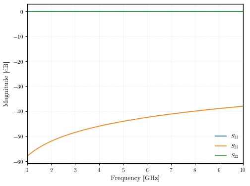
- qpdk.models.electrical_short_2_port(f=5000000000.0)[source]#
Electrical short 2-port connection Sax model.
- Parameters:
f (Annotated[Array | ndarray | Annotated[Annotated[int | integer, PlainValidator(func=~sax.saxtypes.core.val_int, json_schema_input_type=~typing.Any)] | float | floating, PlainValidator(func=~sax.saxtypes.core.val_float, json_schema_input_type=~typing.Any)], floating, PlainValidator(func=~sax.saxtypes.core.val_float_array, json_schema_input_type=~typing.Any)]) – Array of frequency points in Hz
- Returns:
S-parameters dictionary
- Return type:
sax.SDict
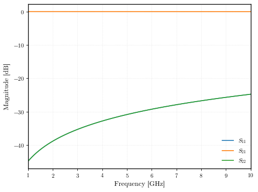
(Source code, svg, pdf, png)

qpdk.models.electrical_short_2_port() S-parameters for \(f\in[1,10]\,\mathrm{GHz}\).#
flipmon#
- qpdk.models.flipmon(f=5000000000.0, capacitance=1e-13, inductance=7e-09, ground_capacitance=0.0)[source]#
LC resonator model for a flipmon qubit.
This model is identical to
double_island_transmon().- Returns:
S-parameters dictionary.
- Return type:
sax.SType
- Parameters:
f (Annotated[Array | ndarray | Annotated[Annotated[int | integer, PlainValidator(func=~sax.saxtypes.core.val_int, json_schema_input_type=~typing.Any)] | float | floating, PlainValidator(func=~sax.saxtypes.core.val_float, json_schema_input_type=~typing.Any)], floating, PlainValidator(func=~sax.saxtypes.core.val_float_array, json_schema_input_type=~typing.Any)])
capacitance (float)
inductance (float)
ground_capacitance (float)
(Source code, svg, pdf, png)

qpdk.models.flipmon() S-parameters for \(f\in[1,10]\,\mathrm{GHz}\).#
flipmon_with_bbox#
- qpdk.models.flipmon_with_bbox(f=5000000000.0, capacitance=1e-13, inductance=7e-09, ground_capacitance=0.0)[source]#
LC resonator model for a flipmon qubit with bounding box ports.
This model is the same as
flipmon().- Returns:
S-parameters dictionary.
- Return type:
sax.SType
- Parameters:
f (Annotated[Array | ndarray | Annotated[Annotated[int | integer, PlainValidator(func=~sax.saxtypes.core.val_int, json_schema_input_type=~typing.Any)] | float | floating, PlainValidator(func=~sax.saxtypes.core.val_float, json_schema_input_type=~typing.Any)], floating, PlainValidator(func=~sax.saxtypes.core.val_float_array, json_schema_input_type=~typing.Any)])
capacitance (float)
inductance (float)
ground_capacitance (float)
(Source code, svg, pdf, png)

qpdk.models.flipmon_with_bbox() S-parameters for \(f\in[1,10]\,\mathrm{GHz}\).#
flipmon_with_resonator#
- qpdk.models.flipmon_with_resonator(f=5000000000.0, qubit_capacitance=1e-13, qubit_inductance=1e-09, resonator_length=5000.0, resonator_cross_section='cpw', coupling_capacitance=1e-14)[source]#
Model for a flipmon qubit coupled to a quarter-wave resonator.
This model is identical to
qubit_with_resonator()but the qubit is set to floating.- Returns:
S-parameters dictionary.
- Return type:
sax.SDict
- Parameters:
f (Annotated[Array | ndarray | Annotated[Annotated[int | integer, PlainValidator(func=~sax.saxtypes.core.val_int, json_schema_input_type=~typing.Any)] | float | floating, PlainValidator(func=~sax.saxtypes.core.val_float, json_schema_input_type=~typing.Any)], floating, PlainValidator(func=~sax.saxtypes.core.val_float_array, json_schema_input_type=~typing.Any)])
qubit_capacitance (float)
qubit_inductance (float)
resonator_length (float)
resonator_cross_section (str)
coupling_capacitance (float)
(Source code, svg, pdf, png)

qpdk.models.flipmon_with_resonator() S-parameters for \(f\in[1,10]\,\mathrm{GHz}\).#
fluxonium#
- qpdk.models.fluxonium(f=5000000000.0, capacitance=1e-14, josephson_inductance=1e-08, superinductance=5e-07, ground_capacitance=0.0)[source]#
S-parameter model for a fluxonium qubit.
A fluxonium qubit consists of a Josephson junction shunted by a large superinductance and a capacitor. In the linear regime, this is modeled as a parallel LCL circuit.
For an accurate microwave model reflecting the real physical layout, the circuit is treated as ungrounded (floating) with optional symmetric parasitic capacitances connecting both ends to ground [NLS+19].

Note
The total shunt capacitance capacitance should include the pads, junction capacitance, and parasitic meander capacitance. Spurious array self-resonance (SR) modes can be phenomenologically modeled by adding to the shunt capacitance or using a multimode model.
- Parameters:
f (Annotated[Array | ndarray | Annotated[Annotated[int | integer, PlainValidator(func=~sax.saxtypes.core.val_int, json_schema_input_type=~typing.Any)] | float | floating, PlainValidator(func=~sax.saxtypes.core.val_float, json_schema_input_type=~typing.Any)], floating, PlainValidator(func=~sax.saxtypes.core.val_float_array, json_schema_input_type=~typing.Any)]) – Array of frequency points in Hz.
capacitance (float) – Total shunt capacitance \(C_\Sigma\) in Farads.
josephson_inductance (float) – Josephson inductance \(L_\text{J}\) in Henries.
superinductance (float) – Superinductance \(L_\text{s}\) in Henries.
ground_capacitance (float) – Parasitic capacitance to ground \(C_g\) at each port in Farads.
- Returns:
S-parameters dictionary with ports o1 and o2.
- Return type:
sax.SDict
(Source code, svg, pdf, png)

qpdk.models.fluxonium() S-parameters for \(f\in[1,10]\,\mathrm{GHz}\).#
fluxonium_coupled#
- qpdk.models.fluxonium_coupled(f=5000000000.0, capacitance=1e-14, josephson_inductance=1e-08, superinductance=5e-07, ground_capacitance=0.0, coupling_capacitance=1e-14, coupling_inductance=0.0)[source]#
Coupled fluxonium qubit model.
This model adds a coupling network to the fluxonium model.
- Parameters:
f (Annotated[Array | ndarray | Annotated[Annotated[int | integer, PlainValidator(func=~sax.saxtypes.core.val_int, json_schema_input_type=~typing.Any)] | float | floating, PlainValidator(func=~sax.saxtypes.core.val_float, json_schema_input_type=~typing.Any)], floating, PlainValidator(func=~sax.saxtypes.core.val_float_array, json_schema_input_type=~typing.Any)]) – Array of frequency points in Hz.
capacitance (float) – Total shunt capacitance \(C_\Sigma\) in Farads.
josephson_inductance (float) – Josephson inductance \(L_\text{J}\) in Henries.
superinductance (float) – Superinductance \(L_\text{s}\) in Henries.
ground_capacitance (float) – Parasitic capacitance to ground \(C_g\) in Farads.
coupling_capacitance (float) – Coupling capacitance \(C_c\) in Farads.
coupling_inductance (float) – Coupling inductance \(L_c\) in Henries.
- Returns:
S-parameters dictionary with ports o1 and o2.
- Return type:
sax.SDict
(Source code, svg, pdf, png)

qpdk.models.fluxonium_coupled() S-parameters for \(f\in[1,10]\,\mathrm{GHz}\).#
fluxonium_with_bbox#
- qpdk.models.fluxonium_with_bbox(f=5000000000.0, capacitance=1e-14, josephson_inductance=1e-08, superinductance=5e-07, ground_capacitance=0.0)[source]#
S-parameter model for a fluxonium qubit with bounding box ports.
This model is the same as
fluxonium().- Returns:
S-parameters dictionary.
- Return type:
sax.SType
- Parameters:
f (Annotated[Array | ndarray | Annotated[Annotated[int | integer, PlainValidator(func=~sax.saxtypes.core.val_int, json_schema_input_type=~typing.Any)] | float | floating, PlainValidator(func=~sax.saxtypes.core.val_float, json_schema_input_type=~typing.Any)], floating, PlainValidator(func=~sax.saxtypes.core.val_float_array, json_schema_input_type=~typing.Any)])
capacitance (float)
josephson_inductance (float)
superinductance (float)
ground_capacitance (float)
(Source code, svg, pdf, png)

qpdk.models.fluxonium_with_bbox() S-parameters for \(f\in[1,10]\,\mathrm{GHz}\).#
fluxonium_with_resonator#
- qpdk.models.fluxonium_with_resonator(f=5000000000.0, capacitance=1e-14, josephson_inductance=1e-08, superinductance=5e-07, ground_capacitance=0.0, resonator_length=5000.0, resonator_cross_section='cpw', coupling_capacitance=1e-14)[source]#
Model for a fluxonium qubit coupled to a quarter-wave resonator.
- Parameters:
f (Annotated[Array | ndarray | Annotated[Annotated[int | integer, PlainValidator(func=~sax.saxtypes.core.val_int, json_schema_input_type=~typing.Any)] | float | floating, PlainValidator(func=~sax.saxtypes.core.val_float, json_schema_input_type=~typing.Any)], floating, PlainValidator(func=~sax.saxtypes.core.val_float_array, json_schema_input_type=~typing.Any)]) – Array of frequency points in Hz.
capacitance (float) – Total shunt capacitance \(C_\Sigma\) in Farads.
josephson_inductance (float) – Josephson inductance \(L_\text{J}\) in Henries.
superinductance (float) – Superinductance \(L_\text{s}\) in Henries.
ground_capacitance (float) – Parasitic capacitance to ground \(C_g\) in Farads.
resonator_length (float) – Length of the quarter-wave resonator in µm.
resonator_cross_section (str) – Cross-section specification for the resonator.
coupling_capacitance (float) – Coupling capacitance between qubit and resonator in Farads.
- Returns:
S-parameters dictionary.
- Return type:
sax.SDict
(Source code, svg, pdf, png)

qpdk.models.fluxonium_with_resonator() S-parameters for \(f\in[1,10]\,\mathrm{GHz}\).#
indium_bump#
- qpdk.models.indium_bump(f=5000000000.0, bump_height=10.0)[source]#
S-parameter model for an indium bump, wrapped to
straight().TODO: add a constant loss channel for indium bumps.
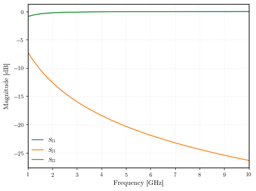
(Source code, svg, pdf, png)

qpdk.models.indium_bump() S-parameters for \(f\in[1,10]\,\mathrm{GHz}\).#
interdigital_capacitor#
- qpdk.models.interdigital_capacitor(*, f=5000000000.0, fingers=4, finger_length=20.0, finger_gap=2.0, thickness=5.0, cross_section='cpw')[source]#
Interdigital capacitor Sax model.
- Parameters:
f (Annotated[Array | ndarray | Annotated[Annotated[int | integer, PlainValidator(func=~sax.saxtypes.core.val_int, json_schema_input_type=~typing.Any)] | float | floating, PlainValidator(func=~sax.saxtypes.core.val_float, json_schema_input_type=~typing.Any)], floating, PlainValidator(func=~sax.saxtypes.core.val_float_array, json_schema_input_type=~typing.Any)]) – Array of frequency points in Hz
fingers (int) – Total number of fingers (must be >= 2)
finger_length (float) – Length of each finger in μm
finger_gap (float) – Gap between adjacent fingers in μm
thickness (float) – Thickness of fingers in μm
cross_section (CrossSectionSpec) – Cross-section specification
- Returns:
S-parameters dictionary
- Return type:
sax.SDict
(Source code, svg, pdf, png)

qpdk.models.interdigital_capacitor() S-parameters for \(f\in[1,10]\,\mathrm{GHz}\).#
josephson_junction#
- qpdk.models.josephson_junction(*, f=5000000000.0, ic=1e-06, capacitance=5e-15, resistance=10000.0, ib=0.0)[source]#
Josephson junction (RCSJ) small-signal Sax model.
Linearized RCSJ model consisting of a bias-dependent Josephson inductance in parallel with capacitance and resistance.
Valid in the superconducting (zero-voltage) state and for small AC signals.
Default capacitance taken from [SFS+15].
See [McC68] for details.
- Parameters:
f (Annotated[Array | ndarray | Annotated[Annotated[int | integer, PlainValidator(func=~sax.saxtypes.core.val_int, json_schema_input_type=~typing.Any)] | float | floating, PlainValidator(func=~sax.saxtypes.core.val_float, json_schema_input_type=~typing.Any)], floating, PlainValidator(func=~sax.saxtypes.core.val_float_array, json_schema_input_type=~typing.Any)]) – Array of frequency points in Hz
ic (Annotated[float | floating, PlainValidator(func=~sax.saxtypes.core.val_float, json_schema_input_type=~typing.Any)]) – Critical current \(I_c\) in Amperes
capacitance (Annotated[float | floating, PlainValidator(func=~sax.saxtypes.core.val_float, json_schema_input_type=~typing.Any)]) – Junction capacitance \(C\) in Farads
resistance (Annotated[float | floating, PlainValidator(func=~sax.saxtypes.core.val_float, json_schema_input_type=~typing.Any)]) – Shunt resistance \(R\) in Ohms
ib (Annotated[float | floating, PlainValidator(func=~sax.saxtypes.core.val_float, json_schema_input_type=~typing.Any)]) – DC bias current \(I_b\) in Amperes (\(\|I_b\| < I_c\))
- Returns:
S-parameters dictionary
- Return type:
sax.SDict
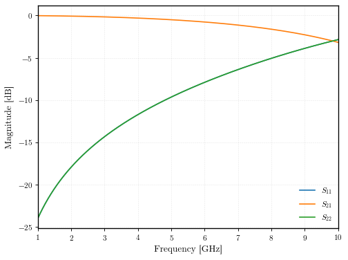
(Source code, svg, pdf, png)

qpdk.models.josephson_junction() S-parameters for \(f\in[1,10]\,\mathrm{GHz}\).#
launcher#
- qpdk.models.launcher(f=5000000000.0, straight_length=200.0, taper_length=100.0, cross_section_big=None, cross_section_small='cpw')[source]#
S-parameter model for a launcher, effectively a straight section followed by a taper.
- Parameters:
f (Array | ndarray | bool | number | bool | int | float | complex | TypedNdArray) – Array of frequency points in Hz
straight_length (Annotated[float | floating, PlainValidator(func=~sax.saxtypes.core.val_float, json_schema_input_type=~typing.Any)]) – Length of the straight section in µm.
taper_length (Annotated[float | floating, PlainValidator(func=~sax.saxtypes.core.val_float, json_schema_input_type=~typing.Any)]) – Length of the taper section in µm.
cross_section_big (CrossSectionSpec | None) – Cross-section for the wide section.
cross_section_small (CrossSectionSpec) – Cross-section for the narrow section.
- Returns:
S-parameters dictionary
- Return type:
sax.SDict
lc_resonator#
- qpdk.models.lc_resonator(f=5000000000.0, capacitance=1e-13, inductance=1e-09, grounded=False, ground_capacitance=0.0)[source]#
LC resonator Sax model with capacitor and inductor in parallel.
The resonance frequency is given by:
If grounded=True, a 2-port short is connected to port o2:

Optional ground capacitances Cg can be added to both ports:
 \[f_r = \frac{1}{2 \pi \sqrt{LC}}\]
For theory and relation to superconductors, see [Gao08].
- Parameters:
f (Annotated[Array | ndarray | Annotated[Annotated[int | integer, PlainValidator(func=~sax.saxtypes.core.val_int, json_schema_input_type=~typing.Any)] | float | floating, PlainValidator(func=~sax.saxtypes.core.val_float, json_schema_input_type=~typing.Any)], floating, PlainValidator(func=~sax.saxtypes.core.val_float_array, json_schema_input_type=~typing.Any)]) – Array of frequency points in Hz.
capacitance (float) – Capacitance of the resonator in Farads.
inductance (float) – Inductance of the resonator in Henries.
grounded (bool) – If True, add a 2-port ground to the second port.
ground_capacitance (float) – Parasitic capacitance to ground Cg at each port in Farads.
- Returns:
S-parameters dictionary with ports o1 and o2.
- Return type:
sax.SDict
(Source code, svg, pdf, png)

qpdk.models.lc_resonator() S-parameters for \(f\in[1,10]\,\mathrm{GHz}\).#
lc_resonator_coupled#
- qpdk.models.lc_resonator_coupled(f=5000000000.0, capacitance=1e-13, inductance=1e-09, grounded=False, ground_capacitance=0.0, coupling_capacitance=1e-14, coupling_inductance=0.0)[source]#
Coupled LC resonator Sax model.
This model extends the basic LC resonator by adding a coupling network consisting of a parallel capacitor and inductor connected in series to one port of the LC resonator.
The resonance frequency of the main LC resonator is given by:
\[f_r = \frac{1}{2 \pi \sqrt{LC}}\]The coupling network modifies the effective coupling to the resonator.

Where \(L_\text{c}\) and \(C_\text{c}\) are the coupling inductance and capacitance, respectively.
- Parameters:
f (Annotated[Array | ndarray | Annotated[Annotated[int | integer, PlainValidator(func=~sax.saxtypes.core.val_int, json_schema_input_type=~typing.Any)] | float | floating, PlainValidator(func=~sax.saxtypes.core.val_float, json_schema_input_type=~typing.Any)], floating, PlainValidator(func=~sax.saxtypes.core.val_float_array, json_schema_input_type=~typing.Any)]) – Array of frequency points in Hz.
capacitance (float) – Capacitance of the main resonator in Farads.
inductance (float) – Inductance of the main resonator in Henries.
grounded (bool) – If True, the resonator is grounded.
ground_capacitance (float) – Parasitic capacitance to ground Cg at each port in Farads.
coupling_capacitance (float) – Coupling capacitance in Farads.
coupling_inductance (float) – Coupling inductance in Henries.
- Returns:
S-parameters dictionary with ports o1 and o2.
- Return type:
sax.SDict
(Source code, svg, pdf, png)

qpdk.models.lc_resonator_coupled() S-parameters for \(f\in[1,10]\,\mathrm{GHz}\).#
lumped_element_resonator#
- qpdk.models.lumped_element_resonator(*, f=5000000000.0, fingers=20, finger_length=20.0, finger_gap=2.0, finger_thickness=5.0, n_turns=5, sheet_inductance=4e-13, cross_section='meander_inductor_cross_section', grounded=False)[source]#
Lumped-element LC resonator SAX model.
Combines an interdigital capacitor and a meander inductor in parallel to form an LC resonator. The resonance frequency is:
\[f_r = \frac{1}{2\pi\sqrt{LC}}\]where \(C\) is computed from the interdigital capacitor geometry using
interdigital_capacitor_capacitance_analytical()and \(L\) is computed from the meander inductor geometry usingmeander_inductor_inductance_analytical().The inductor section uses the width and gap derived from the cross_section to ensure consistent RF behavior across the meander. The vertical spacing between meander runs is set to twice the etch gap to prevent overlap of the etched regions.
- Parameters:
f (Annotated[Array | ndarray | Annotated[Annotated[int | integer, PlainValidator(func=~sax.saxtypes.core.val_int, json_schema_input_type=~typing.Any)] | float | floating, PlainValidator(func=~sax.saxtypes.core.val_float, json_schema_input_type=~typing.Any)], floating, PlainValidator(func=~sax.saxtypes.core.val_float_array, json_schema_input_type=~typing.Any)]) – Array of frequency points in Hz.
fingers (int) – Number of interdigital capacitor fingers.
finger_length (float) – Length of each capacitor finger in µm.
finger_gap (float) – Gap between adjacent capacitor fingers in µm.
finger_thickness (float) – Width of each capacitor finger in µm.
n_turns (int) – Number of horizontal meander inductor runs (must be odd to match the cell geometry where the path spans left-to-right bus bars).
sheet_inductance (float) – Sheet inductance per square in H/□.
cross_section (CrossSectionSpec) – Cross-section specification. Used for substrate permittivity and to determine inductor wire width and gap.
grounded (bool) – If True, one port of the resonator is grounded.
- Returns:
S-parameters dictionary with ports o1 and o2.
- Return type:
sax.SDict
(Source code, svg, pdf, png)

qpdk.models.lumped_element_resonator() S-parameters for \(f\in[1,10]\,\mathrm{GHz}\).#
meander_inductor#
- qpdk.models.meander_inductor(*, f=5000000000.0, n_turns=5, turn_length=200.0, cross_section='meander_inductor_cross_section', sheet_inductance=4e-13)[source]#
Meander inductor SAX model.
Computes the inductance from the meander geometry and returns S-parameters of an equivalent lumped inductor.
The model extracts the center conductor width and gap from the provided cross-section. To ensure the etched regions of adjacent meander runs do not overlap and interfere with the characteristic impedance of each other, the vertical pitch is calculated as:
\[p = w + 2 \cdot g\]where \(w\) is the center conductor width and \(g\) is the gap width. This corresponds to a metal-to-metal spacing of \(2g\).
- Parameters:
f (Annotated[Array | ndarray | Annotated[Annotated[int | integer, PlainValidator(func=~sax.saxtypes.core.val_int, json_schema_input_type=~typing.Any)] | float | floating, PlainValidator(func=~sax.saxtypes.core.val_float, json_schema_input_type=~typing.Any)], floating, PlainValidator(func=~sax.saxtypes.core.val_float_array, json_schema_input_type=~typing.Any)]) – Array of frequency points in Hz.
n_turns (int) – Number of horizontal meander runs.
turn_length (float) – Length of each horizontal run in µm.
cross_section (CrossSectionSpec) – Cross-section specification for the meander wire. Used to determine the wire width and the gap between runs.
sheet_inductance (float) – Sheet inductance per square in H/□.
- Returns:
S-parameters dictionary.
- Return type:
sax.SDict
(Source code, svg, pdf, png)

qpdk.models.meander_inductor() S-parameters for \(f\in[1,10]\,\mathrm{GHz}\).#
meander_inductor_inductance_analytical#
- qpdk.models.meander_inductor_inductance_analytical(n_turns, turn_length, wire_width, wire_gap, sheet_inductance, thickness=None)[source]#
Analytical formula for meander inductor inductance.
The total inductance is the sum of geometric and kinetic contributions:
\[L_{\text{total}} = L_g + L_k\]The geometric inductance \(L_g\) is calculated by summing the self-inductances of all horizontal segments and the mutual inductances between all pairs of parallel segments, following [CSD+23]:
\[L_g = N L_s + 2 \sum_{k=1}^{N-1} (N-k) (-1)^k L_m(k p)\]where \(N\) is the number of turns and \(p\) is the pitch.
The kinetic inductance \(L_k\) is calculated from the sheet inductance \(L_\square\):
\[L_k = L_\square \cdot \frac{\ell_{\text{total}}}{w}\]- Parameters:
n_turns (int) – Number of horizontal meander runs.
turn_length (float) – Length of each horizontal run in µm.
wire_width (float) – Width of the meander wire in µm.
wire_gap (float) – Gap between adjacent meander runs in µm.
sheet_inductance (float) – Sheet inductance per square in H/□.
thickness (float | None) – Thickness of the metal film in µm. If None, it is fetched from the PDK technology parameters.
- Returns:
Total inductance in Henries.
- Return type:
measurement_induced_dephasing#
- qpdk.models.measurement_induced_dephasing(χ_ghz, κ_ghz, n_bar)[source]#
Estimate measurement-induced dephasing rate.
During dispersive readout, photons in the resonator cause additional dephasing of the qubit [BGGW21, GBS+06]:
\[\Gamma_\phi = \frac{8 \chi^2 \bar{n}}{\kappa}\]where \(\bar{n}\) is the mean photon number in the resonator.
- Parameters:
- Returns:
Measurement-induced dephasing rate in GHz.
- Return type:
Example
>>> Γ_φ = measurement_induced_dephasing(-0.001, 0.001, 5.0)
>>> print(f"Γ_φ = {Γ_φ * 1e6:.1f} kHz")
microstrip_epsilon_eff#
- qpdk.models.microstrip_epsilon_eff(w, h, ep_r)[source]#
Effective permittivity of a microstrip line.
Uses the Hammerstad-Jensen formula as given in Pozar.
\[\varepsilon_{\mathrm{eff}} = \frac{\varepsilon_r + 1}{2} + \frac{\varepsilon_r - 1}{2} \left(\frac{1}{\sqrt{1 + 12h/w}} + 0.04(1 - w/h)^2 \Theta(1 - w/h)\right)\]where the last term contributes only for narrow strips (\(w/h < 1\)).
References
Hammerstad & Jensen; Pozar, Eqs. 3.195-3.196.
- Parameters:
w (Annotated[Array | ndarray | Annotated[Annotated[int | integer, PlainValidator(func=~sax.saxtypes.core.val_int, json_schema_input_type=~typing.Any)] | float | floating, PlainValidator(func=~sax.saxtypes.core.val_float, json_schema_input_type=~typing.Any)], floating, PlainValidator(func=~sax.saxtypes.core.val_float_array, json_schema_input_type=~typing.Any)]) – Strip width (m).
h (Annotated[Array | ndarray | Annotated[Annotated[int | integer, PlainValidator(func=~sax.saxtypes.core.val_int, json_schema_input_type=~typing.Any)] | float | floating, PlainValidator(func=~sax.saxtypes.core.val_float, json_schema_input_type=~typing.Any)], floating, PlainValidator(func=~sax.saxtypes.core.val_float_array, json_schema_input_type=~typing.Any)]) – Substrate height (m).
ep_r (Annotated[Array | ndarray | Annotated[Annotated[int | integer, PlainValidator(func=~sax.saxtypes.core.val_int, json_schema_input_type=~typing.Any)] | float | floating, PlainValidator(func=~sax.saxtypes.core.val_float, json_schema_input_type=~typing.Any)], floating, PlainValidator(func=~sax.saxtypes.core.val_float_array, json_schema_input_type=~typing.Any)]) – Relative permittivity of the substrate.
- Returns:
Effective permittivity (dimensionless).
- Return type:
microstrip_thickness_correction#
- qpdk.models.microstrip_thickness_correction(w, h, t, ep_r, ep_eff)[source]#
Conductor thickness correction for a microstrip line.
Uses the widely-adopted Schneider correction as presented in Pozar and Gupta et al.
\[\begin{split}\begin{aligned} w_e &= w + \frac{t}{\pi} \ln\frac{4e}{\sqrt{(t/h)^2 + (t/(wPI + 1.1tPI))^2}} \\ \varepsilon_{\mathrm{eff},t} &= \varepsilon_{\mathrm{eff}} - \frac{(\varepsilon_r - 1)\,t/h} {4.6\,\sqrt{w/h}} \end{aligned}\end{split}\]Then the corrected \(Z_0\) is computed with the effective width \(w_e\) and corrected \(\varepsilon_{\mathrm{eff},t}\).
References
Pozar, §3.8; Gupta, Garg, Bahl & Bhartia
- Parameters:
w (Annotated[Array | ndarray | Annotated[Annotated[int | integer, PlainValidator(func=~sax.saxtypes.core.val_int, json_schema_input_type=~typing.Any)] | float | floating, PlainValidator(func=~sax.saxtypes.core.val_float, json_schema_input_type=~typing.Any)], floating, PlainValidator(func=~sax.saxtypes.core.val_float_array, json_schema_input_type=~typing.Any)]) – Strip width (m).
h (Annotated[Array | ndarray | Annotated[Annotated[int | integer, PlainValidator(func=~sax.saxtypes.core.val_int, json_schema_input_type=~typing.Any)] | float | floating, PlainValidator(func=~sax.saxtypes.core.val_float, json_schema_input_type=~typing.Any)], floating, PlainValidator(func=~sax.saxtypes.core.val_float_array, json_schema_input_type=~typing.Any)]) – Substrate height (m).
t (Annotated[Array | ndarray | Annotated[Annotated[int | integer, PlainValidator(func=~sax.saxtypes.core.val_int, json_schema_input_type=~typing.Any)] | float | floating, PlainValidator(func=~sax.saxtypes.core.val_float, json_schema_input_type=~typing.Any)], floating, PlainValidator(func=~sax.saxtypes.core.val_float_array, json_schema_input_type=~typing.Any)]) – Conductor thickness (m).
ep_r (Annotated[Array | ndarray | Annotated[Annotated[int | integer, PlainValidator(func=~sax.saxtypes.core.val_int, json_schema_input_type=~typing.Any)] | float | floating, PlainValidator(func=~sax.saxtypes.core.val_float, json_schema_input_type=~typing.Any)], floating, PlainValidator(func=~sax.saxtypes.core.val_float_array, json_schema_input_type=~typing.Any)]) – Relative permittivity of the substrate.
ep_eff (Annotated[Array | ndarray | Annotated[Annotated[int | integer, PlainValidator(func=~sax.saxtypes.core.val_int, json_schema_input_type=~typing.Any)] | float | floating, PlainValidator(func=~sax.saxtypes.core.val_float, json_schema_input_type=~typing.Any)], floating, PlainValidator(func=~sax.saxtypes.core.val_float_array, json_schema_input_type=~typing.Any)]) – Uncorrected effective permittivity.
- Returns:
(w_eff, ep_eff_t, z0_t)— effective width (m), thickness-corrected effective permittivity, and characteristic impedance (Ω).- Return type:
microstrip_z0#
- qpdk.models.microstrip_z0(w, h, ep_eff)[source]#
Characteristic impedance of a microstrip line.
Uses the Hammerstad-Jensen approximation as given in Pozar.
\[\begin{split}\begin{aligned} Z_0 = \begin{cases} \displaystyle\frac{60}{\sqrt{\varepsilon_{\mathrm{eff}}}} \ln\!\left(\frac{8h}{w} + \frac{w}{4h}\right) & w/h \le 1 \\[6pt] \displaystyle\frac{120\pi} {\sqrt{\varepsilon_{\mathrm{eff}}}\, \bigl[w/h + 1.393 + 0.667\ln(w/h + 1.444)\bigr]} & w/h \ge 1 \end{cases} \end{aligned}\end{split}\]References
Hammerstad & Jensen; Pozar, Eqs. 3.197-3.198.
- Parameters:
w (Annotated[Array | ndarray | Annotated[Annotated[int | integer, PlainValidator(func=~sax.saxtypes.core.val_int, json_schema_input_type=~typing.Any)] | float | floating, PlainValidator(func=~sax.saxtypes.core.val_float, json_schema_input_type=~typing.Any)], floating, PlainValidator(func=~sax.saxtypes.core.val_float_array, json_schema_input_type=~typing.Any)]) – Strip width (m).
h (Annotated[Array | ndarray | Annotated[Annotated[int | integer, PlainValidator(func=~sax.saxtypes.core.val_int, json_schema_input_type=~typing.Any)] | float | floating, PlainValidator(func=~sax.saxtypes.core.val_float, json_schema_input_type=~typing.Any)], floating, PlainValidator(func=~sax.saxtypes.core.val_float_array, json_schema_input_type=~typing.Any)]) – Substrate height (m).
ep_eff (Annotated[Array | ndarray | Annotated[Annotated[int | integer, PlainValidator(func=~sax.saxtypes.core.val_int, json_schema_input_type=~typing.Any)] | float | floating, PlainValidator(func=~sax.saxtypes.core.val_float, json_schema_input_type=~typing.Any)], floating, PlainValidator(func=~sax.saxtypes.core.val_float_array, json_schema_input_type=~typing.Any)]) – Effective permittivity (see
microstrip_epsilon_eff()).
- Returns:
Characteristic impedance (Ω).
- Return type:
nxn#
- qpdk.models.nxn(f=5000000000.0, west=1, east=1, north=1, south=1)[source]#
NxN junction model using tee components.
This model creates an N-port divider/combiner by chaining 3-port tee junctions. All ports are connected to a single node.
- Parameters:
f (Annotated[Array | ndarray | Annotated[Annotated[int | integer, PlainValidator(func=~sax.saxtypes.core.val_int, json_schema_input_type=~typing.Any)] | float | floating, PlainValidator(func=~sax.saxtypes.core.val_float, json_schema_input_type=~typing.Any)], floating, PlainValidator(func=~sax.saxtypes.core.val_float_array, json_schema_input_type=~typing.Any)]) – Array of frequency points in Hz.
west (int) – Number of ports on the west side.
east (int) – Number of ports on the east side.
north (int) – Number of ports on the north side.
south (int) – Number of ports on the south side.
- Returns:
S-parameters dictionary with ports o1, o2, …, oN.
- Return type:
sax.SType
- Raises:
ValueError – If total number of ports is not positive.
(Source code, svg, pdf, png)

qpdk.models.nxn() S-parameters for \(f\in[1,10]\,\mathrm{GHz}\).#
open#
- qpdk.models.open(*, f=5000000000.0, n_ports=1)#
Electrical open connection Sax model.
Useful for specifying some ports to remain open while not exposing them for connections in circuits.
- Parameters:
f (Annotated[Array | ndarray | Annotated[Annotated[int | integer, PlainValidator(func=~sax.saxtypes.core.val_int, json_schema_input_type=~typing.Any)] | float | floating, PlainValidator(func=~sax.saxtypes.core.val_float, json_schema_input_type=~typing.Any)], floating, PlainValidator(func=~sax.saxtypes.core.val_float_array, json_schema_input_type=~typing.Any)]) – Array of frequency points in Hz
n_ports (int) – Number of ports to set as opened
- Returns:
S-dictionary where \(S = I_\text{n_ports}\)
- Return type:
dict[tuple[Annotated[str, PlainValidator(func=~sax.saxtypes.singlemode.val_port, json_schema_input_type=~typing.Any)], Annotated[str, PlainValidator(func=~sax.saxtypes.singlemode.val_port, json_schema_input_type=~typing.Any)]], Annotated[Array, complexfloating, PlainValidator(func=~sax.saxtypes.core.val_complex_array, json_schema_input_type=~typing.Any)]] | dict[tuple[Annotated[str, PlainValidator(func=~sax.saxtypes.multimode.val_port_mode, json_schema_input_type=~typing.Any)], Annotated[str, PlainValidator(func=~sax.saxtypes.multimode.val_port_mode, json_schema_input_type=~typing.Any)]], Annotated[Array, complexfloating, PlainValidator(func=~sax.saxtypes.core.val_complex_array, json_schema_input_type=~typing.Any)]]
References
Pozar
(Source code, svg, pdf, png)

qpdk.models.open() S-parameters for \(f\in[1,10]\,\mathrm{GHz}\).#
plate_capacitor#
- qpdk.models.plate_capacitor(*, f=5000000000.0, length=26.0, width=5.0, gap=7.0, cross_section='cpw')[source]#
Plate capacitor Sax model.
- Parameters:
f (Annotated[Array | ndarray | Annotated[Annotated[int | integer, PlainValidator(func=~sax.saxtypes.core.val_int, json_schema_input_type=~typing.Any)] | float | floating, PlainValidator(func=~sax.saxtypes.core.val_float, json_schema_input_type=~typing.Any)], floating, PlainValidator(func=~sax.saxtypes.core.val_float_array, json_schema_input_type=~typing.Any)]) – Array of frequency points in Hz
length (float) – Length of the capacitor pad in μm
width (float) – Width of the capacitor pad in μm
gap (float) – Gap between plates in μm
cross_section (CrossSectionSpec) – Cross-section specification
- Returns:
S-parameters dictionary
- Return type:
sax.SDict
(Source code, svg, pdf, png)

qpdk.models.plate_capacitor() S-parameters for \(f\in[1,10]\,\mathrm{GHz}\).#
propagation_constant#
- qpdk.models.propagation_constant(f, ep_eff, tand=0.0, ep_r=1.0)[source]#
Complex propagation constant of a quasi-TEM transmission line.
For the general lossy case
\[\gamma = \alpha_d + j\,\beta\]where the dielectric attenuation is
\[\alpha_d = \frac{\pi f}{C_M_S} \frac{\varepsilon_r}{\sqrt{\varepsilon_{\mathrm{eff}}}} \frac{\varepsilon_{\mathrm{eff}} - 1} {\varepsilon_r - 1} \tan\delta\]and the phase constant is
\[\beta = \frac{2\pi f}{C_M_S}\,\sqrt{\varepsilon_{\mathrm{eff}}}\]For a superconducting line (\(\tan\delta = 0\)) the propagation is purely imaginary: \(\gamma = j\beta\).
References
Pozar, §3.8
- Parameters:
f (Annotated[Array | ndarray | Annotated[Annotated[int | integer, PlainValidator(func=~sax.saxtypes.core.val_int, json_schema_input_type=~typing.Any)] | float | floating, PlainValidator(func=~sax.saxtypes.core.val_float, json_schema_input_type=~typing.Any)], floating, PlainValidator(func=~sax.saxtypes.core.val_float_array, json_schema_input_type=~typing.Any)]) – Frequency (Hz).
ep_eff (Annotated[Array | ndarray | Annotated[Annotated[int | integer, PlainValidator(func=~sax.saxtypes.core.val_int, json_schema_input_type=~typing.Any)] | float | floating, PlainValidator(func=~sax.saxtypes.core.val_float, json_schema_input_type=~typing.Any)], floating, PlainValidator(func=~sax.saxtypes.core.val_float_array, json_schema_input_type=~typing.Any)]) – Effective permittivity.
tand (Annotated[Array | ndarray | Annotated[Annotated[int | integer, PlainValidator(func=~sax.saxtypes.core.val_int, json_schema_input_type=~typing.Any)] | float | floating, PlainValidator(func=~sax.saxtypes.core.val_float, json_schema_input_type=~typing.Any)], floating, PlainValidator(func=~sax.saxtypes.core.val_float_array, json_schema_input_type=~typing.Any)]) – Dielectric loss tangent (default 0 — lossless).
ep_r (Annotated[Array | ndarray | Annotated[Annotated[int | integer, PlainValidator(func=~sax.saxtypes.core.val_int, json_schema_input_type=~typing.Any)] | float | floating, PlainValidator(func=~sax.saxtypes.core.val_float, json_schema_input_type=~typing.Any)], floating, PlainValidator(func=~sax.saxtypes.core.val_float_array, json_schema_input_type=~typing.Any)]) – Substrate relative permittivity (only needed when
tand > 0).
- Returns:
Complex propagation constant \(\gamma\) (1/m).
- Return type:
purcell_decay_rate#
- qpdk.models.purcell_decay_rate(g_ghz, ω_t_ghz, ω_r_ghz, κ_ghz)[source]#
Estimate the Purcell decay rate of a transmon through a resonator.
The Purcell effect limits qubit lifetime when coupled to a lossy resonator. In the dispersive regime [BGGW21, HSJ+08]:
\[\gamma_\text{Purcell} = \kappa \left(\frac{g}{\Delta}\right)^2\]where \(\kappa\) is the resonator decay rate and \(\Delta = \omega_t - \omega_r\).
- Parameters:
g_ghz (float | TypeAliasForwardRef('ArrayLike')) – Coupling strength in GHz.
ω_t_ghz (float | TypeAliasForwardRef('ArrayLike')) – Transmon frequency in GHz.
ω_r_ghz (float | TypeAliasForwardRef('ArrayLike')) – Resonator frequency in GHz.
κ_ghz (float | TypeAliasForwardRef('ArrayLike')) – Resonator linewidth (decay rate) in GHz.
- Returns:
Purcell decay rate in GHz.
- Return type:
Example
>>> γ = purcell_decay_rate(0.1, 5.0, 7.0, 0.001)
>>> T_purcell = 1 / (γ * 1e9)
>>> print(f"T_Purcell = {T_purcell * 1e6:.0f} µs")
quarter_wave_resonator_coupled#
- qpdk.models.quarter_wave_resonator_coupled(f=5000000000.0, length=5000.0, coupling_gap=0.27, coupling_straight_length=20, cross_section='cpw')[source]#
Model for a quarter-wave coplanar waveguide resonator coupled to a probeline.
- Parameters:
cross_section (CrossSectionSpec) – The cross-section of the CPW.
f (Annotated[Array | ndarray | Annotated[Annotated[int | integer, PlainValidator(func=~sax.saxtypes.core.val_int, json_schema_input_type=~typing.Any)] | float | floating, PlainValidator(func=~sax.saxtypes.core.val_float, json_schema_input_type=~typing.Any)], floating, PlainValidator(func=~sax.saxtypes.core.val_float_array, json_schema_input_type=~typing.Any)]) – Frequency in Hz at which to evaluate the S-parameters.
length (float) – Total length of the resonator in μm.
coupling_gap (float) – Gap between the resonator and the probeline in μm.
coupling_straight_length (float) – Length of the coupling section in μm.
- Returns:
S-parameters dictionary
- Return type:
sax.SDict
(Source code, svg, pdf, png)

qpdk.models.quarter_wave_resonator_coupled() S-parameters for \(f\in[1,10]\,\mathrm{GHz}\).#
qubit_with_resonator#
- qpdk.models.qubit_with_resonator(f=5000000000.0, qubit_capacitance=1e-13, qubit_inductance=1e-09, qubit_grounded=False, resonator_length=5000.0, resonator_cross_section='cpw', coupling_capacitance=1e-14)[source]#
Model for a transmon qubit coupled to a quarter-wave resonator.
This model corresponds to the layout function
transmon_with_resonator().The model combines: - A transmon qubit (LC resonator) - A quarter-wave coplanar waveguide resonator - A coupling capacitor connecting the qubit to the resonator

The qubit can be either: - A double-island transmon (
qubit_grounded=False): both islands floating - A shunted transmon (qubit_grounded=True): one island groundedUse
ec_to_capacitance()andej_to_inductance()to convert from qubit Hamiltonian parameters (\(E_C\), \(E_J\)) to circuit parameters.Note
This function is not JIT-compiled because it depends on
straight_shorted(), which internally uses cpw_parameters for transmission line modeling.- Parameters:
f (Annotated[Array | ndarray | Annotated[Annotated[int | integer, PlainValidator(func=~sax.saxtypes.core.val_int, json_schema_input_type=~typing.Any)] | float | floating, PlainValidator(func=~sax.saxtypes.core.val_float, json_schema_input_type=~typing.Any)], floating, PlainValidator(func=~sax.saxtypes.core.val_float_array, json_schema_input_type=~typing.Any)]) – Array of frequency points in Hz.
qubit_capacitance (float) – Total capacitance \(C_\Sigma\) of the qubit in Farads. Convert from charging energy using
ec_to_capacitance().qubit_inductance (float) – Josephson inductance \(L_\text{J}\) in Henries. Convert from Josephson energy using
ej_to_inductance().qubit_grounded (bool) – If True, the qubit is a shunted transmon (grounded). If False, it is a double-island transmon (ungrounded).
resonator_length (float) – Length of the quarter-wave resonator in µm.
resonator_cross_section (str) – Cross-section specification for the resonator.
coupling_capacitance (float) – Coupling capacitance between qubit and resonator in Farads. Use
coupling_strength_to_capacitance()to convert from qubit-resonator coupling strength \(g\).
- Returns:
- S-parameters dictionary with ports
o1(resonator input) and
o2(qubit ground or floating).
- S-parameters dictionary with ports
- Return type:
sax.SDict
(Source code, svg, pdf, png)

qpdk.models.qubit_with_resonator() S-parameters for \(f\in[1,10]\,\mathrm{GHz}\).#
rectangle#
- qpdk.models.rectangle(f=5000000000.0, length=1000, cross_section='cpw')[source]#
S-parameter model for a rectangular section, wrapped to
straight().- Parameters:
f (Annotated[Array | ndarray | Annotated[Annotated[int | integer, PlainValidator(func=~sax.saxtypes.core.val_int, json_schema_input_type=~typing.Any)] | float | floating, PlainValidator(func=~sax.saxtypes.core.val_float, json_schema_input_type=~typing.Any)], floating, PlainValidator(func=~sax.saxtypes.core.val_float_array, json_schema_input_type=~typing.Any)]) – Array of frequency points in Hz
length (Annotated[float | floating, PlainValidator(func=~sax.saxtypes.core.val_float, json_schema_input_type=~typing.Any)]) – Physical length in µm
cross_section (CrossSectionSpec) – The cross-section of the waveguide.
- Returns:
S-parameters dictionary
- Return type:
sax.SDict
(Source code, svg, pdf, png)

qpdk.models.rectangle() S-parameters for \(f\in[1,10]\,\mathrm{GHz}\).#
resonator#
- qpdk.models.resonator(f=5000000000.0, length=1000, cross_section='cpw')[source]#
S-parameter model for a simple transmission line resonator.
- Parameters:
f (Annotated[Array | ndarray | Annotated[Annotated[int | integer, PlainValidator(func=~sax.saxtypes.core.val_int, json_schema_input_type=~typing.Any)] | float | floating, PlainValidator(func=~sax.saxtypes.core.val_float, json_schema_input_type=~typing.Any)], floating, PlainValidator(func=~sax.saxtypes.core.val_float_array, json_schema_input_type=~typing.Any)]) – Array of frequency points in Hz
length (Annotated[float | floating, PlainValidator(func=~sax.saxtypes.core.val_float, json_schema_input_type=~typing.Any)]) – Physical length in µm
cross_section (CrossSectionSpec) – The cross-section of the waveguide.
- Returns:
S-parameters dictionary
- Return type:
sax.SType
(Source code, svg, pdf, png)

qpdk.models.resonator() S-parameters for \(f\in[1,10]\,\mathrm{GHz}\).#
resonator_coupled#
- qpdk.models.resonator_coupled(f=5000000000.0, length=5000.0, coupling_gap=0.27, coupling_straight_length=20, cross_section='cpw', open_start=True, open_end=False)[source]#
Model for a coplanar waveguide resonator coupled to a probeline.
- Parameters:
cross_section (CrossSectionSpec) – The cross-section of the CPW.
f (Annotated[Array | ndarray | Annotated[Annotated[int | integer, PlainValidator(func=~sax.saxtypes.core.val_int, json_schema_input_type=~typing.Any)] | float | floating, PlainValidator(func=~sax.saxtypes.core.val_float, json_schema_input_type=~typing.Any)], floating, PlainValidator(func=~sax.saxtypes.core.val_float_array, json_schema_input_type=~typing.Any)]) – Frequency in Hz at which to evaluate the S-parameters.
length (float) – Total length of the resonator in μm.
coupling_gap (float) – Gap between the resonator and the probeline in μm.
coupling_straight_length (float) – Length of the coupling section in μm.
open_start (bool) – If True, adds an electrical open at the start.
open_end (bool) – If True, adds an electrical open at the end.
- Returns:
S-parameters dictionary with 4 ports.
- Return type:
sax.SDict
(Source code, svg, pdf, png)

qpdk.models.resonator_coupled() S-parameters for \(f\in[1,10]\,\mathrm{GHz}\).#
resonator_frequency#
- qpdk.models.resonator_frequency(*, length, epsilon_eff=None, media=None, cross_section='cpw', is_quarter_wave=True)[source]#
Calculate the resonance frequency of a quarter- or half-wave CPW resonator.
\[\begin{split}\begin{aligned} f &= \frac{v_p}{4L} \mathtt{ (quarter-wave resonator)} \\ f &= \frac{v_p}{2L} \mathtt{ (half-wave resonator)} \end{aligned}\end{split}\]The phase velocity is \(v_p = c_0 / \sqrt{\varepsilon_{\mathrm{eff}}}\).
See [MP12, Sim01] for details.
- Parameters:
length (float) – Length of the resonator in μm.
epsilon_eff (float | None) – Effective permittivity. If
None(default), computed from cross_section usingcpw_parameters().media (Any) – Deprecated. Use epsilon_eff or cross_section instead.
cross_section (CrossSectionSpec) – Cross-section specification (used only when epsilon_eff and media are not provided).
is_quarter_wave (bool) – If True, calculates for a quarter-wave resonator; if False, for a half-wave resonator. default is True.
- Returns:
Resonance frequency in Hz.
- Return type:
resonator_half_wave#
- qpdk.models.resonator_half_wave(f=5000000000.0, length=1000, cross_section='cpw')[source]#
S-parameter model for a half-wave resonator (open at both ends).
- Parameters:
f (Annotated[Array | ndarray | Annotated[Annotated[int | integer, PlainValidator(func=~sax.saxtypes.core.val_int, json_schema_input_type=~typing.Any)] | float | floating, PlainValidator(func=~sax.saxtypes.core.val_float, json_schema_input_type=~typing.Any)], floating, PlainValidator(func=~sax.saxtypes.core.val_float_array, json_schema_input_type=~typing.Any)]) – Array of frequency points in Hz
length (Annotated[float | floating, PlainValidator(func=~sax.saxtypes.core.val_float, json_schema_input_type=~typing.Any)]) – Physical length in µm
cross_section (CrossSectionSpec) – The cross-section of the waveguide.
- Returns:
S-parameters dictionary
- Return type:
sax.SType
(Source code, svg, pdf, png)

qpdk.models.resonator_half_wave() S-parameters for \(f\in[1,10]\,\mathrm{GHz}\).#
resonator_linewidth_from_q#
- qpdk.models.resonator_linewidth_from_q(ω_r_ghz, q_ext)[source]#
Compute resonator linewidth from external quality factor.
Converts external quality factor to linewidth (half-linewidth at half-maximum) [GopplFB+08, MP12]:
\[\kappa = \frac{\omega_r}{Q_\text{ext}}\]- Parameters:
- Returns:
Resonator linewidth \(\kappa\) in GHz.
- Return type:
Example
>>> κ = resonator_linewidth_from_q(7.0, 10_000)
>>> print(f"κ = {κ * 1e6:.1f} kHz")
resonator_quarter_wave#
- qpdk.models.resonator_quarter_wave(f=5000000000.0, length=1000, cross_section='cpw')[source]#
S-parameter model for a quarter-wave resonator (shorted at one end).
- Parameters:
f (Annotated[Array | ndarray | Annotated[Annotated[int | integer, PlainValidator(func=~sax.saxtypes.core.val_int, json_schema_input_type=~typing.Any)] | float | floating, PlainValidator(func=~sax.saxtypes.core.val_float, json_schema_input_type=~typing.Any)], floating, PlainValidator(func=~sax.saxtypes.core.val_float_array, json_schema_input_type=~typing.Any)]) – Array of frequency points in Hz
length (Annotated[float | floating, PlainValidator(func=~sax.saxtypes.core.val_float, json_schema_input_type=~typing.Any)]) – Physical length in µm
cross_section (CrossSectionSpec) – The cross-section of the waveguide.
- Returns:
S-parameters dictionary
- Return type:
sax.SType
(Source code, svg, pdf, png)

qpdk.models.resonator_quarter_wave() S-parameters for \(f\in[1,10]\,\mathrm{GHz}\).#
series_impedance#
- qpdk.models.series_impedance(f=5000000000.0, z=0.0, z0=50.0)[source]#
Two-port series impedance Sax model.

See [MP12] (Ch. 4, Table 4.1, Table 4.2, Problem 4.11) for the S-parameter derivation.
- Parameters:
f (Annotated[Array | ndarray | Annotated[Annotated[int | integer, PlainValidator(func=~sax.saxtypes.core.val_int, json_schema_input_type=~typing.Any)] | float | floating, PlainValidator(func=~sax.saxtypes.core.val_float, json_schema_input_type=~typing.Any)], floating, PlainValidator(func=~sax.saxtypes.core.val_float_array, json_schema_input_type=~typing.Any)]) – Array of frequency points in Hz.
z (Annotated[float | floating, PlainValidator(func=~sax.saxtypes.core.val_float, json_schema_input_type=~typing.Any)]) – Complex impedance in Ohms.
z0 (float) – Reference characteristic impedance in Ohms.
- Returns:
S-parameters dictionary with ports o1 and o2.
- Return type:
sax.SDict
short#
- qpdk.models.short(*, f=5000000000.0, n_ports=1)#
Electrical short connection Sax model.
- Parameters:
f (Annotated[Array | ndarray | Annotated[Annotated[int | integer, PlainValidator(func=~sax.saxtypes.core.val_int, json_schema_input_type=~typing.Any)] | float | floating, PlainValidator(func=~sax.saxtypes.core.val_float, json_schema_input_type=~typing.Any)], floating, PlainValidator(func=~sax.saxtypes.core.val_float_array, json_schema_input_type=~typing.Any)]) – Array of frequency points in Hz
n_ports (int) – Number of ports to set as shorted
- Returns:
S-dictionary where \(S = -I_\text{n_ports}\)
- Return type:
dict[tuple[Annotated[str, PlainValidator(func=~sax.saxtypes.singlemode.val_port, json_schema_input_type=~typing.Any)], Annotated[str, PlainValidator(func=~sax.saxtypes.singlemode.val_port, json_schema_input_type=~typing.Any)]], Annotated[Array, complexfloating, PlainValidator(func=~sax.saxtypes.core.val_complex_array, json_schema_input_type=~typing.Any)]] | dict[tuple[Annotated[str, PlainValidator(func=~sax.saxtypes.multimode.val_port_mode, json_schema_input_type=~typing.Any)], Annotated[str, PlainValidator(func=~sax.saxtypes.multimode.val_port_mode, json_schema_input_type=~typing.Any)]], Annotated[Array, complexfloating, PlainValidator(func=~sax.saxtypes.core.val_complex_array, json_schema_input_type=~typing.Any)]]
References
Pozar
(Source code, svg, pdf, png)

qpdk.models.short() S-parameters for \(f\in[1,10]\,\mathrm{GHz}\).#
short_2_port#
- qpdk.models.short_2_port(f=5000000000.0)#
Electrical short 2-port connection Sax model.
- Parameters:
f (Annotated[Array | ndarray | Annotated[Annotated[int | integer, PlainValidator(func=~sax.saxtypes.core.val_int, json_schema_input_type=~typing.Any)] | float | floating, PlainValidator(func=~sax.saxtypes.core.val_float, json_schema_input_type=~typing.Any)], floating, PlainValidator(func=~sax.saxtypes.core.val_float_array, json_schema_input_type=~typing.Any)]) – Array of frequency points in Hz
- Returns:
S-parameters dictionary
- Return type:
sax.SDict
(Source code, svg, pdf, png)

qpdk.models.short_2_port() S-parameters for \(f\in[1,10]\,\mathrm{GHz}\).#
shunt_admittance#
- qpdk.models.shunt_admittance(f=5000000000.0, y=0.0, z0=50.0)[source]#
Two-port shunt admittance Sax model.

See [MP12] (Ch. 4, Table 4.1, Table 4.2, Problem 4.11) for the S-parameter derivation.
- Parameters:
f (Annotated[Array | ndarray | Annotated[Annotated[int | integer, PlainValidator(func=~sax.saxtypes.core.val_int, json_schema_input_type=~typing.Any)] | float | floating, PlainValidator(func=~sax.saxtypes.core.val_float, json_schema_input_type=~typing.Any)], floating, PlainValidator(func=~sax.saxtypes.core.val_float_array, json_schema_input_type=~typing.Any)]) – Array of frequency points in Hz.
y (Annotated[float | floating, PlainValidator(func=~sax.saxtypes.core.val_float, json_schema_input_type=~typing.Any)]) – Complex admittance in Siemens.
z0 (float) – Reference characteristic impedance in Ohms.
- Returns:
S-parameters dictionary with ports o1 and o2.
- Return type:
sax.SDict
shunted_transmon#
- qpdk.models.shunted_transmon(f=5000000000.0, capacitance=1e-13, inductance=7e-09, ground_capacitance=0.0)[source]#
LC resonator model for a shunted transmon qubit.
A shunted transmon has one island grounded and the other island connected to the junction. This is modeled as a grounded parallel LC resonator.
The qubit frequency is approximately:
\[f_q \approx \frac{1}{2\pi} \sqrt{8 E_J E_C} - E_C\]For the LC model, the resonance frequency is:
\[f_r = \frac{1}{2\pi\sqrt{LC}}\]Use
ec_to_capacitance()andej_to_inductance()to convert from qubit Hamiltonian parameters.
- Parameters:
f (Annotated[Array | ndarray | Annotated[Annotated[int | integer, PlainValidator(func=~sax.saxtypes.core.val_int, json_schema_input_type=~typing.Any)] | float | floating, PlainValidator(func=~sax.saxtypes.core.val_float, json_schema_input_type=~typing.Any)], floating, PlainValidator(func=~sax.saxtypes.core.val_float_array, json_schema_input_type=~typing.Any)]) – Array of frequency points in Hz.
capacitance (float) – Total capacitance \(C_\Sigma\) of the qubit in Farads.
inductance (float) – Josephson inductance \(L_\text{J}\) in Henries.
ground_capacitance (float) – Parasitic capacitance to ground \(C_g\) at the floating port in Farads.
- Returns:
S-parameters dictionary with ports o1 and o2.
- Return type:
sax.SDict
(Source code, svg, pdf, png)

qpdk.models.shunted_transmon() S-parameters for \(f\in[1,10]\,\mathrm{GHz}\).#
squid_junction#
- qpdk.models.squid_junction(*, f=5000000000.0, ic_tot=2e-06, asymmetry=0.0, capacitance=1e-14, resistance=5000.0, ib=0.0, flux=0.0)[source]#
DC SQUID small-signal Sax model in the zero-screening limit.
Treats the DC SQUID as a single effective RCSJ whose critical current is tunable by an external magnetic flux. Assumes negligible loop geometric inductance.
See [KYG+07] and [Tin15] for details on asymmetric SQUIDs and effective Josephson inductance.
- Parameters:
f (Annotated[Array | ndarray | Annotated[Annotated[int | integer, PlainValidator(func=~sax.saxtypes.core.val_int, json_schema_input_type=~typing.Any)] | float | floating, PlainValidator(func=~sax.saxtypes.core.val_float, json_schema_input_type=~typing.Any)], floating, PlainValidator(func=~sax.saxtypes.core.val_float_array, json_schema_input_type=~typing.Any)]) – Array of frequency points in Hz
ic_tot (Annotated[float | floating, PlainValidator(func=~sax.saxtypes.core.val_float, json_schema_input_type=~typing.Any)]) – Total critical current sum \(I_{c1} + I_{c2}\) in Amperes
asymmetry (Annotated[float | floating, PlainValidator(func=~sax.saxtypes.core.val_float, json_schema_input_type=~typing.Any)]) – Junction asymmetry \((I_{c1} - I_{c2}) / I_{c,tot}\)
capacitance (Annotated[float | floating, PlainValidator(func=~sax.saxtypes.core.val_float, json_schema_input_type=~typing.Any)]) – Total SQUID capacitance \(C_1 + C_2\) in Farads
resistance (Annotated[float | floating, PlainValidator(func=~sax.saxtypes.core.val_float, json_schema_input_type=~typing.Any)]) – Total SQUID shunt resistance \(R_1 || R_2\) in Ohms
ib (Annotated[float | floating, PlainValidator(func=~sax.saxtypes.core.val_float, json_schema_input_type=~typing.Any)]) – DC bias current \(I_b\) in Amperes
flux (Annotated[float | floating, PlainValidator(func=~sax.saxtypes.core.val_float, json_schema_input_type=~typing.Any)]) – External magnetic flux \(\Phi_{ext}\) in Webers
- Returns:
S-parameters dictionary
- Return type:
sax.SDict
(Source code, svg, pdf, png)

qpdk.models.squid_junction() S-parameters for \(f\in[1,10]\,\mathrm{GHz}\).#
straight#
- qpdk.models.straight(f=5000000000.0, length=1000, cross_section='cpw')[source]#
S-parameter model for a straight coplanar waveguide.
Wraps
sax.models.rf.coplanar_waveguide(), extracting the physical dimensions from the given cross_section and the PDK layer stack.Computes S-parameters analytically using conformal-mapping CPW theory following Simons [Sim01] (ch. 2) and the Qucs-S CPW model (Qucs technical documentation, §12.4). Conductor thickness corrections use the first-order model of Gupta, Garg, Bahl, and Bhartia [GGBB96].
- Parameters:
f (Annotated[Array | ndarray | Annotated[Annotated[int | integer, PlainValidator(func=~sax.saxtypes.core.val_int, json_schema_input_type=~typing.Any)] | float | floating, PlainValidator(func=~sax.saxtypes.core.val_float, json_schema_input_type=~typing.Any)], floating, PlainValidator(func=~sax.saxtypes.core.val_float_array, json_schema_input_type=~typing.Any)]) – Array of frequency points in Hz
length (Annotated[float | floating, PlainValidator(func=~sax.saxtypes.core.val_float, json_schema_input_type=~typing.Any)]) – Physical length in µm
cross_section (CrossSectionSpec) – The cross-section of the waveguide.
- Returns:
S-parameters dictionary
- Return type:
sax.SDict
(Source code, svg, pdf, png)
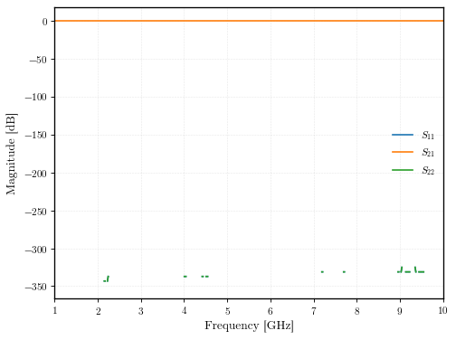

qpdk.models.straight() S-parameters for \(f\in[1,10]\,\mathrm{GHz}\).#
straight_all_angle#
- qpdk.models.straight_all_angle(f=5000000000.0, length=1000, cross_section='cpw')[source]#
S-parameter model for a straight coplanar waveguide.
Same as
straight().- Parameters:
f (Annotated[Array | ndarray | Annotated[Annotated[int | integer, PlainValidator(func=~sax.saxtypes.core.val_int, json_schema_input_type=~typing.Any)] | float | floating, PlainValidator(func=~sax.saxtypes.core.val_float, json_schema_input_type=~typing.Any)], floating, PlainValidator(func=~sax.saxtypes.core.val_float_array, json_schema_input_type=~typing.Any)]) – Array of frequency points in Hz
length (Annotated[float | floating, PlainValidator(func=~sax.saxtypes.core.val_float, json_schema_input_type=~typing.Any)]) – Physical length in µm
cross_section (CrossSectionSpec) – The cross-section of the waveguide.
- Returns:
S-parameters dictionary
- Return type:
sax.SDict
(Source code, svg, pdf, png)
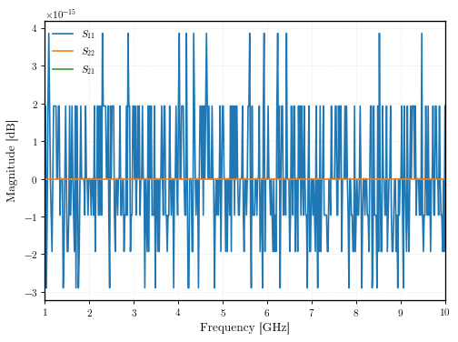

qpdk.models.straight_all_angle() S-parameters for \(f\in[1,10]\,\mathrm{GHz}\).#
straight_double_open#
- qpdk.models.straight_double_open(f=5000000000.0, length=1000, cross_section='cpw')[source]#
S-parameter model for a straight waveguide with open ends.
Note
Ports
o1ando2are internally open-circuited and should not be used. They are provided to match the number of ports in the layout component.- Parameters:
f (Annotated[Array | ndarray | Annotated[Annotated[int | integer, PlainValidator(func=~sax.saxtypes.core.val_int, json_schema_input_type=~typing.Any)] | float | floating, PlainValidator(func=~sax.saxtypes.core.val_float, json_schema_input_type=~typing.Any)], floating, PlainValidator(func=~sax.saxtypes.core.val_float_array, json_schema_input_type=~typing.Any)]) – Array of frequency points in Hz
length (Annotated[float | floating, PlainValidator(func=~sax.saxtypes.core.val_float, json_schema_input_type=~typing.Any)]) – Physical length in µm
cross_section (CrossSectionSpec) – The cross-section of the waveguide.
- Returns:
S-parameters dictionary
- Return type:
sax.SType
(Source code, svg, pdf, png)
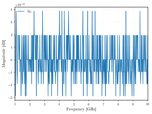

qpdk.models.straight_double_open() S-parameters for \(f\in[1,10]\,\mathrm{GHz}\).#
straight_microstrip#
- qpdk.models.straight_microstrip(f=5000000000.0, length=1000, width=10.0, h=500.0, t=0.2, ep_r=11.45, tand=0.0)[source]#
S-parameter model for a straight microstrip transmission line.
Wraps
sax.models.rf.microstrip(), mapping the qpdk parameter names to the upstream model.Computes S-parameters analytically using the Hammerstad-Jensen [HJ80] closed-form expressions for effective permittivity and characteristic impedance, as described in Pozar [MP12] (ch. 3, §3.8). Conductor thickness corrections follow Gupta et al. [GGBB96] (§2.2.4).
- Parameters:
f (Annotated[Array | ndarray | Annotated[Annotated[int | integer, PlainValidator(func=~sax.saxtypes.core.val_int, json_schema_input_type=~typing.Any)] | float | floating, PlainValidator(func=~sax.saxtypes.core.val_float, json_schema_input_type=~typing.Any)], floating, PlainValidator(func=~sax.saxtypes.core.val_float_array, json_schema_input_type=~typing.Any)]) – Array of frequency points in Hz.
length (Annotated[float | floating, PlainValidator(func=~sax.saxtypes.core.val_float, json_schema_input_type=~typing.Any)]) – Physical length in µm.
width (Annotated[float | floating, PlainValidator(func=~sax.saxtypes.core.val_float, json_schema_input_type=~typing.Any)]) – Strip width in µm.
h (Annotated[float | floating, PlainValidator(func=~sax.saxtypes.core.val_float, json_schema_input_type=~typing.Any)]) – Substrate height in µm.
t (Annotated[float | floating, PlainValidator(func=~sax.saxtypes.core.val_float, json_schema_input_type=~typing.Any)]) – Conductor thickness in µm (default 0.2 µm = 200 nm).
ep_r (Annotated[float | floating, PlainValidator(func=~sax.saxtypes.core.val_float, json_schema_input_type=~typing.Any)]) – Relative permittivity of the substrate (default 11.45 for Si).
tand (Annotated[float | floating, PlainValidator(func=~sax.saxtypes.core.val_float, json_schema_input_type=~typing.Any)]) – Dielectric loss tangent (default 0 — lossless).
- Returns:
S-parameters dictionary.
- Return type:
sax.SDict
(Source code, svg, pdf, png)
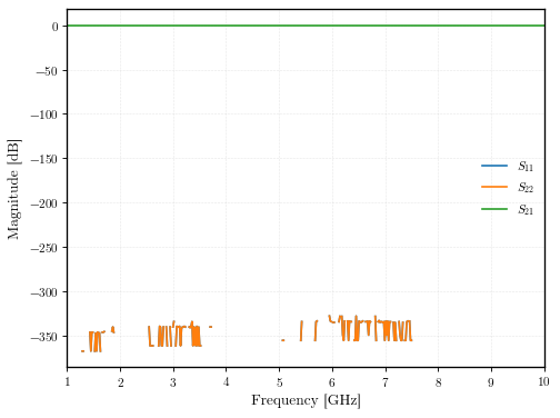

qpdk.models.straight_microstrip() S-parameters for \(f\in[1,10]\,\mathrm{GHz}\).#
straight_open#
- qpdk.models.straight_open(f=5000000000.0, length=1000, cross_section='cpw')[source]#
S-parameter model for a straight waveguide with one open end.
Note
The port
o2is internally open-circuited and should not be used. It is provided to match the number of ports in the layout component.- Parameters:
f (Annotated[Array | ndarray | Annotated[Annotated[int | integer, PlainValidator(func=~sax.saxtypes.core.val_int, json_schema_input_type=~typing.Any)] | float | floating, PlainValidator(func=~sax.saxtypes.core.val_float, json_schema_input_type=~typing.Any)], floating, PlainValidator(func=~sax.saxtypes.core.val_float_array, json_schema_input_type=~typing.Any)]) – Array of frequency points in Hz
length (Annotated[float | floating, PlainValidator(func=~sax.saxtypes.core.val_float, json_schema_input_type=~typing.Any)]) – Physical length in µm
cross_section (CrossSectionSpec) – The cross-section of the waveguide.
- Returns:
S-parameters dictionary
- Return type:
sax.SType
(Source code, svg, pdf, png)

qpdk.models.straight_open() S-parameters for \(f\in[1,10]\,\mathrm{GHz}\).#
straight_shorted#
- qpdk.models.straight_shorted(f=5000000000.0, length=1000, cross_section='cpw')[source]#
S-parameter model for a straight waveguide with one shorted end.
This may be used to model a quarter-wave coplanar waveguide resonator.
Note
The port
o2is internally shorted and should not be used. It seems to be a Sax limitation that we need to define at least two ports.- Parameters:
f (Annotated[Array | ndarray | Annotated[Annotated[int | integer, PlainValidator(func=~sax.saxtypes.core.val_int, json_schema_input_type=~typing.Any)] | float | floating, PlainValidator(func=~sax.saxtypes.core.val_float, json_schema_input_type=~typing.Any)], floating, PlainValidator(func=~sax.saxtypes.core.val_float_array, json_schema_input_type=~typing.Any)]) – Array of frequency points in Hz
length (Annotated[float | floating, PlainValidator(func=~sax.saxtypes.core.val_float, json_schema_input_type=~typing.Any)]) – Physical length in µm
cross_section (CrossSectionSpec) – The cross-section of the waveguide.
- Returns:
S-parameters dictionary
- Return type:
sax.SDict
(Source code, svg, pdf, png)

qpdk.models.straight_shorted() S-parameters for \(f\in[1,10]\,\mathrm{GHz}\).#
taper_cross_section#
- qpdk.models.taper_cross_section(f=5000000000.0, length=1000, cross_section_1='cpw', cross_section_2='cpw', n_points=50)[source]#
S-parameter model for a cross-section taper using linear interpolation.
- Parameters:
f (Array | ndarray | bool | number | bool | int | float | complex | TypedNdArray) – Array of frequency points in Hz
length (Annotated[float | floating, PlainValidator(func=~sax.saxtypes.core.val_float, json_schema_input_type=~typing.Any)]) – Physical length in µm
cross_section_1 (CrossSectionSpec) – Cross-section for the start of the taper.
cross_section_2 (CrossSectionSpec) – Cross-section for the end of the taper.
n_points (int) – Number of segments to divide the taper into for simulation.
- Returns:
S-parameters dictionary
- Return type:
sax.SDict
(Source code, svg, pdf, png)

qpdk.models.taper_cross_section() S-parameters for \(f\in[1,10]\,\mathrm{GHz}\).#
transmission_line_s_params#
- qpdk.models.transmission_line_s_params(gamma, z0, length, z_ref=None)[source]#
S-parameters of a uniform transmission line (ABCD→S conversion).
The ABCD matrix of a line with characteristic impedance \(Z_0\), propagation constant \(\gamma\), and length \(\ell\) is:
\[\begin{split}\begin{aligned} \begin{pmatrix} A & B \\ C & D \end{pmatrix} = \begin{pmatrix} \cosh\theta & Z_0\sinh\theta \\ \sinh\theta / Z_0 & \cosh\theta \end{pmatrix}, \quad \theta = \gamma\ell \end{aligned}\end{split}\]Converting to S-parameters referenced to \(Z_{\mathrm{ref}}\)
\[\begin{split}\begin{aligned} S_{11} &= \frac{A + B/Z_{\mathrm{ref}} - CZ_{\mathrm{ref}} - D}{ A + B/Z_{\mathrm{ref}} + CZ_{\mathrm{ref}} + D} \\ S_{21} &= \frac{2}{A + B/Z_{\mathrm{ref}} + CZ_{\mathrm{ref}} + D} \end{aligned}\end{split}\]When
z_refisNonethe reference impedance defaults toz0(matched case), giving \(S_{11} = 0\) and \(S_{21} = e^{-\gamma\ell}\).References
Pozar, Table 4.2
- Parameters:
gamma (Annotated[Annotated[Annotated[int | integer, PlainValidator(func=~sax.saxtypes.core.val_int, json_schema_input_type=~typing.Any)] | float | floating, PlainValidator(func=~sax.saxtypes.core.val_float, json_schema_input_type=~typing.Any)] | complex | inexact, PlainValidator(func=~sax.saxtypes.core.val_complex, json_schema_input_type=~typing.Any)]) – Complex propagation constant (1/m).
z0 (Annotated[Annotated[Annotated[int | integer, PlainValidator(func=~sax.saxtypes.core.val_int, json_schema_input_type=~typing.Any)] | float | floating, PlainValidator(func=~sax.saxtypes.core.val_float, json_schema_input_type=~typing.Any)] | complex | inexact, PlainValidator(func=~sax.saxtypes.core.val_complex, json_schema_input_type=~typing.Any)]) – Characteristic impedance (Ω).
length (Annotated[Array | ndarray | Annotated[Annotated[int | integer, PlainValidator(func=~sax.saxtypes.core.val_int, json_schema_input_type=~typing.Any)] | float | floating, PlainValidator(func=~sax.saxtypes.core.val_float, json_schema_input_type=~typing.Any)], floating, PlainValidator(func=~sax.saxtypes.core.val_float_array, json_schema_input_type=~typing.Any)]) – Physical length (m).
z_ref (Annotated[Annotated[Annotated[int | integer, PlainValidator(func=~sax.saxtypes.core.val_int, json_schema_input_type=~typing.Any)] | float | floating, PlainValidator(func=~sax.saxtypes.core.val_float, json_schema_input_type=~typing.Any)] | complex | inexact, PlainValidator(func=~sax.saxtypes.core.val_complex, json_schema_input_type=~typing.Any)] | None) – Reference (port) impedance (Ω). Defaults to
z0.
- Returns:
(S11, S21)— complex S-parameter arrays.- Return type:
transmon_coupled#
- qpdk.models.transmon_coupled(f=5000000000.0, capacitance=1e-13, inductance=1e-09, grounded=False, ground_capacitance=0.0, coupling_capacitance=1e-14, coupling_inductance=0.0)[source]#
Coupled transmon qubit model.
This model extends the basic transmon qubit by adding a coupling network consisting of a parallel capacitor and/or inductor. This can represent capacitive or inductive coupling between qubits or between a qubit and a readout resonator.
The coupling network is connected in series with the LC resonator:

- For capacitive coupling (common for qubit-resonator coupling):
Set
coupling_capacitanceto the coupling capacitor valueSet
coupling_inductance=0.0
- For inductive coupling (common for flux-tunable coupling):
Set
coupling_inductanceto the coupling inductor valueSet
coupling_capacitance=0.0(or small value)
Use
coupling_strength_to_capacitance()to convert from the qubit-resonator coupling strength \(g\) to the coupling capacitance.- Parameters:
f (Annotated[Array | ndarray | Annotated[Annotated[int | integer, PlainValidator(func=~sax.saxtypes.core.val_int, json_schema_input_type=~typing.Any)] | float | floating, PlainValidator(func=~sax.saxtypes.core.val_float, json_schema_input_type=~typing.Any)], floating, PlainValidator(func=~sax.saxtypes.core.val_float_array, json_schema_input_type=~typing.Any)]) – Array of frequency points in Hz.
capacitance (float) – Total capacitance \(C_\Sigma\) of the qubit in Farads.
inductance (float) – Josephson inductance \(L_\text{J}\) in Henries.
grounded (bool) – If True, the qubit is a shunted transmon (grounded). If False, it is a double-pad transmon (ungrounded).
ground_capacitance (float) – Parasitic capacitance to ground \(C_g\) in Farads.
coupling_capacitance (float) – Coupling capacitance \(C_c\) in Farads.
coupling_inductance (float) – Coupling inductance \(L_c\) in Henries.
- Returns:
S-parameters dictionary with ports o1 and o2.
- Return type:
sax.SDict
(Source code, svg, pdf, png)
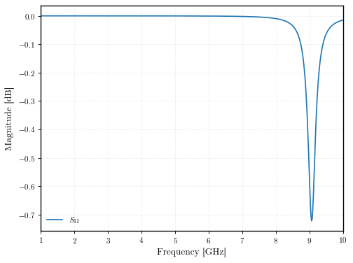

qpdk.models.transmon_coupled() S-parameters for \(f\in[1,10]\,\mathrm{GHz}\).#
transmon_with_resonator#
- qpdk.models.transmon_with_resonator(f=5000000000.0, qubit_capacitance=1e-13, qubit_inductance=1e-09, qubit_grounded=False, resonator_length=5000.0, resonator_cross_section='cpw', coupling_capacitance=1e-14)[source]#
Model for a transmon qubit coupled to a quarter-wave resonator.
This model is identical to
qubit_with_resonator().- Returns:
S-parameters dictionary.
- Return type:
sax.SDict
- Parameters:
f (Annotated[Array | ndarray | Annotated[Annotated[int | integer, PlainValidator(func=~sax.saxtypes.core.val_int, json_schema_input_type=~typing.Any)] | float | floating, PlainValidator(func=~sax.saxtypes.core.val_float, json_schema_input_type=~typing.Any)], floating, PlainValidator(func=~sax.saxtypes.core.val_float_array, json_schema_input_type=~typing.Any)])
qubit_capacitance (float)
qubit_inductance (float)
qubit_grounded (bool)
resonator_length (float)
resonator_cross_section (str)
coupling_capacitance (float)
(Source code, svg, pdf, png)

qpdk.models.transmon_with_resonator() S-parameters for \(f\in[1,10]\,\mathrm{GHz}\).#
tsv#
- qpdk.models.tsv(f=5000000000.0, via_height=1000.0)[source]#
S-parameter model for a through-silicon via (TSV), wrapped to
straight().TODO: add a constant loss channel for TSVs.
(Source code, svg, pdf, png)

qpdk.models.tsv() S-parameters for \(f\in[1,10]\,\mathrm{GHz}\).#
unimon_coupled#
- qpdk.models.unimon_coupled(f=5000000000.0, arm_length=3000.0, cross_section='cpw', junction_capacitance=5e-15, junction_inductance=-7e-09, coupling_capacitance=1e-14)[source]#
SAX model for a capacitively coupled unimon qubit.
The unimon is modeled as a closed system of two shorted quarter-wave CPW resonators connected by a Josephson junction. Interaction with the qubit is provided via a single coupling capacitor connected to one of the arms.

- Parameters:
f (Annotated[Array | ndarray | Annotated[Annotated[int | integer, PlainValidator(func=~sax.saxtypes.core.val_int, json_schema_input_type=~typing.Any)] | float | floating, PlainValidator(func=~sax.saxtypes.core.val_float, json_schema_input_type=~typing.Any)], floating, PlainValidator(func=~sax.saxtypes.core.val_float_array, json_schema_input_type=~typing.Any)]) – Array of frequency points in Hz.
arm_length (float) – Length of each quarter-wave resonator arm in µm.
cross_section (str) – Cross-section specification for the CPW arms.
junction_capacitance (float) – Junction capacitance \(C_J\) in Farads.
junction_inductance (float) – Junction inductance \(L_J\) in Henries.
coupling_capacitance (float) – Coupling capacitance \(C_c\) in Farads.
- Returns:
S-parameters dictionary with a single port
o1.- Return type:
sax.SDict
(Source code, svg, pdf, png)

qpdk.models.unimon_coupled() S-parameters for \(f\in[1,10]\,\mathrm{GHz}\).#
unimon_energies#
- qpdk.models.unimon_energies(ec_ghz=1.0, el_ghz=5.0, ej_ghz=10.0, phi_ext=3.141592653589793, n_max=30, n_levels=5)[source]#
Compute the lowest energy eigenvalues of the unimon Hamiltonian.
Diagonalises the Hamiltonian returned by
unimon_hamiltonian()and returns then_levelslowest eigenvalues, shifted so that the ground state energy is zero.- Parameters:
ec_ghz (float) – Charging energy \(E_C\) in GHz.
el_ghz (float) – Inductive energy \(E_L\) in GHz.
ej_ghz (float) – Josephson energy \(E_J\) in GHz.
phi_ext (float) – External flux \(\varphi_{\text{ext}}\) in radians.
n_max (int) – Charge-basis truncation.
n_levels (int) – Number of lowest energy levels to return.
- Returns:
Array of shape
(n_levels,)with energies in GHz, referenced to the ground state.- Return type:
Example
>>> energies = unimon_energies(ec_ghz=1.0, el_ghz=5.0, ej_ghz=10.0)
>>> f_01 = float(energies[1])  # qubit frequency in GHz
>>> alpha = float(energies[2] - 2 * energies[1])  # anharmonicity
unimon_frequency_and_anharmonicity#
- qpdk.models.unimon_frequency_and_anharmonicity(ec_ghz=1.0, el_ghz=5.0, ej_ghz=10.0, phi_ext=3.141592653589793, n_max=30)[source]#
Compute the qubit transition frequency and anharmonicity of the unimon.
The qubit frequency is
\[f_{01} = E_1 - E_0\]and the anharmonicity is
\[\alpha = (E_2 - E_1) - (E_1 - E_0) = E_2 - 2 E_1\](since \(E_0 = 0\) after shifting).
- Parameters:
- Returns:
Tuple of (frequency_ghz, anharmonicity_ghz).
- Return type:
Example
>>> f01, alpha = unimon_frequency_and_anharmonicity(
...     ec_ghz=1.0, el_ghz=5.0, ej_ghz=10.0
... )
>>> print(f"f_01 = {f01:.3f} GHz, alpha = {alpha:.3f} GHz")
unimon_hamiltonian#
- qpdk.models.unimon_hamiltonian(ec_ghz=1.0, el_ghz=5.0, ej_ghz=10.0, phi_ext=3.141592653589793, n_max=30)[source]#
Build the unimon Hamiltonian matrix in the charge basis.
The effective single-mode unimon Hamiltonian is
\[\hat{H} = 4 E_C \hat{n}^2 + \tfrac{1}{2} E_L (\hat{\varphi} - \varphi_{\text{ext}})^2 - E_J \cos\hat{\varphi}\]Energy Scales and Physics: - \(E_J\): The Josephson energy of the single non-linear junction. - \(E_C\): The effective charging energy. The large geometric capacitance
of the CPW resonator means this is lower than typical transmons.
\(E_L\): The inductive energy provided by the CPW resonator shunting the junction. The unimon operates in the regime \(E_L \sim E_J\).
Similarities to Fluxonium: The effective single-mode circuit model of the unimon is mathematically identical to a fluxonium qubit. The inductive shunt (provided by the CPW resonators) guarantees there are no isolated superconducting islands, making the unimon intrinsically immune to dephasing caused by low-frequency \(1/f\) charge noise.
Phase and Charge Operators: Because the unimon is inductively shunted, its potential energy features a quadratic term \(\tfrac{1}{2} E_L \hat{\varphi}^2\), meaning the potential is not \(2\pi\)-periodic. Thus, the phase operator \(\hat{\varphi}\) must be treated as an extended, non-compact variable. Consequently, the conjugate charge variable \(n\) is continuous, rather than taking discrete integer values as it does for a transmon.
Note on this implementation: To evaluate the Hamiltonian, we use a standard truncated discrete charge basis approximation (\(n \in \{-n_{\max}, \ldots, +n_{\max}\}\)). The charge operator is derived from qutip.charge, and the non-compact phase space operators are approximated as nearest-neighbor hopping matrices.
- Parameters:
ec_ghz (float) – Charging energy \(E_C\) in GHz.
el_ghz (float) – Inductive energy \(E_L\) in GHz.
ej_ghz (float) – Josephson energy \(E_J\) in GHz.
phi_ext (float) – External flux bias \(\varphi_{\text{ext}}\) in radians (reduced flux-quantum units). The optimal operating point is \(\pi\).
n_max (int) – Charge-basis truncation; Hilbert-space dimension is \(2 n_{\max} + 1\).
- Returns:
A
(2*n_max+1, 2*n_max+1)Hermitian matrix (in GHz).- Raises:
ImportError – If the QuTiP extra is not installed.
ModuleNotFoundError – If a dependency other than QuTiP fails to import.
- Return type:
xmon_transmon#
- qpdk.models.xmon_transmon(f=5000000000.0, capacitance=1e-13, inductance=7e-09)[source]#
LC resonator model for an Xmon style transmon qubit.
An Xmon transmon is typically shunted, so this model wraps
shunted_transmon().- Returns:
S-parameters dictionary.
- Return type:
sax.SType
- Parameters:
f (Annotated[Array | ndarray | Annotated[Annotated[int | integer, PlainValidator(func=~sax.saxtypes.core.val_int, json_schema_input_type=~typing.Any)] | float | floating, PlainValidator(func=~sax.saxtypes.core.val_float, json_schema_input_type=~typing.Any)], floating, PlainValidator(func=~sax.saxtypes.core.val_float_array, json_schema_input_type=~typing.Any)])
capacitance (float)
inductance (float)
(Source code, svg, pdf, png)

qpdk.models.xmon_transmon() S-parameters for \(f\in[1,10]\,\mathrm{GHz}\).#
References#
Alexandre Blais, Arne L. Grimsmo, S. M. Girvin, and Andreas Wallraff. Circuit quantum electrodynamics. Reviews of Modern Physics, 93(2):025005, May 2021. doi:10.1103/RevModPhys.93.025005.
Qi-Ming Chen, Priyank Singh, Rostislav Duda, Giacomo Catto, Aarne Keränen, Arman Alizadeh, Timm Mörstedt, Aashish Sah, András Gunyhó, Wei Liu, and Mikko Möttönen. Compact inductor-capacitor resonators at sub-gigahertz frequencies. Physical Review Research, 5(4):043126, November 2023. doi:10.1103/PhysRevResearch.5.043126.
Zijun Chen, A. Megrant, J. Kelly, R. Barends, J. Bochmann, Yu Chen, B. Chiaro, A. Dunsworth, E. Jeffrey, J. Y. Mutus, P. J. J. O'Malley, C. Neill, P. Roushan, D. Sank, A. Vainsencher, J. Wenner, T. C. White, A. N. Cleland, and John M. Martinis. Fabrication and characterization of aluminum airbridges for superconducting microwave circuits. Applied Physics Letters, February 2014. doi:10.1063/1.4863745.
J. Gambetta, A. Blais, D. I. Schuster, A. Wallraff, L. Frunzio, J. Majer, M. H. Devoret, S. M. Girvin, and R. J. Schoelkopf. Qubit-photon interactions in a cavity: measurement-induced dephasing and number splitting. Physical Review A, 74(4):042318, October 2006. doi:10.1103/PhysRevA.74.042318.
Jiansong Gao. The Physics of Superconducting Microwave Resonators. PhD thesis, California Institute of Technology, 2008. doi:10.7907/RAT0-VM75.
Kuldip C. Gupta, R. Garg, I. Bahl, and P. Bhartia. Microstrip Lines and Slotlines. Artech House, Boston, 2. ed edition, 1996. ISBN 978-0-89006-766-6.
M. Göppl, A. Fragner, M. Baur, R. Bianchetti, S. Filipp, J. M. Fink, P. J. Leek, G. Puebla, L. Steffen, and A. Wallraff. Coplanar waveguide resonators for circuit quantum electrodynamics. Journal of Applied Physics, 104(11):113904, December 2008. doi:10.1063/1.3010859.
E. Hammerstad and O. Jensen. Accurate Models for Microstrip Computer-Aided Design. In 1980 IEEE MTT-S International Microwave Symposium Digest, 407–409. Washington, DC, USA, 1980. IEEE. doi:10.1109/MWSYM.1980.1124303.
A. A. Houck, J. A. Schreier, B. R. Johnson, J. M. Chow, Jens Koch, J. M. Gambetta, D. I. Schuster, L. Frunzio, M. H. Devoret, S. M. Girvin, and R. J. Schoelkopf. Controlling the spontaneous emission of a superconducting transmon qubit. Physical Review Letters, 101(8):080502, August 2008. doi:10.1103/PhysRevLett.101.080502.
Eric Hyyppa, Suman Kundu, Chun Fai Chan, András Gunyhó, Juho Hotari, David Janzso, Kristinn Juliusson, Olavi Kiuru, Janne Kotilahti, Alessandro Landra, Wei Liu, Fabian Marxer, Akseli Mäkinen, Jean-Luc Orgiazzi, Mario Partanen, Jukka Räbinä, Joni Rönkkö, Mykhailo Seppälä, Slawomir Simbierowicz, Vasilii Sokolov, Jani Suuronen, Francesca Tozzini, Mikko Tuokkola, Jami Viitanen, Visa Vesterinen, Zijun Zhang, Leif Grönberg, Joonas Govenius, and Mikko Möttönen. Unimon qubit. Nature Communications, 13(1):6895, November 2022. doi:10.1038/s41467-022-34614-w.
Z. Kim, C. P. Vlahacos, J. E. Hoffman, J. A. Grover, K. D. Voigt, B. K. Cooper, C. J. Ballard, B. S. Palmer, M. Hafezi, J. M. Taylor, J. R. Anderson, A. J. Dragt, C. J. Lobb, L. A. Orozco, S. L. Rolston, and F. C. Wellstood. Thin-film superconducting resonator tunable to the ground-state hyperfine splitting of ⁸⁷Rb. AIP Advances, 1(4):042107, December 2011. doi:10.1063/1.3651466.
Jens Koch, Terri M. Yu, Jay Gambetta, A. A. Houck, D. I. Schuster, J. Majer, Alexandre Blais, M. H. Devoret, S. M. Girvin, and R. J. Schoelkopf. Charge-insensitive qubit design derived from the Cooper pair box. Physical Review A, 76(4):042319, October 2007. doi:10.1103/PhysRevA.76.042319.
P. Krantz, M. Kjaergaard, F. Yan, T. P. Orlando, S. Gustavsson, and W. D. Oliver. A quantum engineer's guide to superconducting qubits. Applied Physics Reviews, 6(2):021318, June 2019. doi:10.1063/1.5089550.
David M. Pozar. Microwave Engineering. John Wiley & Sons, Inc., 4 edition, 2012. ISBN 978-0-470-63155-3.
D. E. McCumber. Effect of ac impedance on dc voltage-current characteristics of superconductor weak-link junctions. Journal of Applied Physics, 39(7):3113–3118, June 1968. doi:10.1063/1.1656743.
Long B. Nguyen, Yen-Hsiang Lin, Aaron Somoroff, Raymond Mencia, Nicholas Grabon, and Vladimir E. Manucharyan. High-Coherence Fluxonium Qubit. Physical Review X, 9(4):041041, December 2019. doi:10.1103/PhysRevX.9.041041.
Niko Savola. Design and modelling of long-coherence qubits using energy participation ratios. Master's thesis, Aalto University, February 2023. URN:NBN:fi:aalto-202305213270.
A V Shcherbakova, K G Fedorov, K V Shulga, V V Ryazanov, V V Bolginov, V A Oboznov, S V Egorov, V O Shkolnikov, M J Wolf, D Beckmann, and A V Ustinov. Fabrication and measurements of hybrid Nb/Al Josephson junctions and flux qubits with \mkbibemph \ensuremath \pi -shifters. Superconductor Science and Technology, 28(2):025009, February 2015. doi:10.1088/0953-2048/28/2/025009.
Rainee Simons. Coplanar Waveguide Circuits, Components, and Systems. Number v. 165 in Wiley Series in Microwave and Optical Engineering. Wiley Interscience, New York, 2001. ISBN 978-0-471-46393-1. doi:10.1002/0471224758.
Michael Tinkham. Introduction to Superconductivity. Dover Books on Physics. Dover Publ, Mineola, NY, 2 ed edition, 2015. ISBN 978-0-486-43503-9.
Sasu Tuohino, Vasilii Vadimov, Wallace Teixeira, Tommi Malmelin, Matti Silveri, and Mikko Möttönen. Multimode physics of the unimon circuit. Physical Review Research, 6(3):033001, July 2024. doi:10.1103/PhysRevResearch.6.033001.