

Q2D Cross-Section Impedance of a Coplanar Waveguide#
This notebook demonstrates how to extract the characteristic impedance
:math:Z_0 of a coplanar waveguide (CPW) cross-section using the
Ansys 2D Extractor (Q2D) quasi-static field solver via PyAEDT.
The Q2D solver computes per-unit-length RLGC parameters from the
cross-sectional geometry, from which the characteristic impedance
can be obtained as a function of frequency. We compare the
full-wave Q2D result against the analytical conformal-mapping estimate
from :func:~qpdk.models.cpw.cpw_parameters.
Prerequisites:
Ansys Electronics Desktop installed (requires license)
Install hfss extras:
uv sync --extra hfssorpip install qpdk[hfss]
References:
PyAEDT Documentation: https://aedt.docs.pyansys.com/
Q2D Coplanar Waveguide Example: https://examples.aedt.docs.pyansys.com/version/dev/examples/high_frequency/radiofrequency_mmwave/coplanar_waveguide.html
Simons, Coplanar Waveguide Circuits, Components, and Systems [Sim01]
Setup and Imports#
Initialize Q2D Project#
Set up an Ansys 2D Extractor project. The Q2D solver uses a quasi-static approach to compute per-unit-length transmission-line parameters from the 2D cross-section.
Note: This section requires Ansys Electronics Desktop to be installed and licensed.
# Configuration for Q2D simulation
Q2D_CONFIG = {
    "sweep_start_ghz": 1.0,  # Sweep from 1 GHz
    "sweep_stop_ghz": 10.0,  # to 10 GHz
    "sweep_step_ghz": 0.1,  # 100 MHz step
}
# Ensure Ansys path is set so PyAEDT can find it
ansys_default_path = "/usr/ansys_inc/v252/AnsysEM"
if "ANSYSEM_ROOT252" not in os.environ and Path(ansys_default_path).exists():
    os.environ["ANSYSEM_ROOT252"] = ansys_default_path

settings.use_grpc_uds = False

# Create temporary directory for project
temp_dir = tempfile.TemporaryDirectory(suffix=".ansys_qpdk")
project_path = Path(temp_dir.name) / "cpw_q2d.aedt"

# Initialize Q2D
q2d = Q2d(
    project=str(project_path),
    design="CPW_Impedance",
    non_graphical=False,
    new_desktop=True,
    version="2025.2",
)

print(f"Q2D project created: {q2d.project_file}")
print(f"Design name: {q2d.design_name}")
PyAEDT INFO: Python version 3.12.13 (main, Mar 3 2026, 14:59:34) [Clang 21.1.4 ].
PyAEDT INFO: PyAEDT version 0.26.2.
PyAEDT INFO: Initializing new Desktop session.
PyAEDT INFO: AEDT version 2025.2.
PyAEDT INFO: New AEDT session is starting on gRPC port 57449.
PyAEDT INFO: Starting new AEDT gRPC session on port 57449.
PyAEDT INFO: Launching AEDT server with gRPC transport mode: TransportMode.UDS
PyAEDT INFO: Electronics Desktop started on gRPC port 57449 after 9.2 seconds.
PyAEDT INFO: AEDT installation Path /usr/ansys_inc/v252/AnsysEM
PyAEDT INFO: Connected to AEDT gRPC session on port 57449.
PyAEDT WARNING: Service Pack is not detected. PyAEDT is currently connecting in Insecure Mode.
PyAEDT WARNING: Please download and install latest Service Pack to use connect to AEDT in Secure Mode.
PyAEDT INFO: Project cpw_q2d has been created.
PyAEDT INFO: Added design 'CPW_Impedance' of type 2D Extractor.
PyAEDT INFO: AEDT objects correctly read
Q2D project created: /tmp/tmp70dmm41z.ansys_qpdk/cpw_q2d.aedt
Design name: CPW_Impedance
Build CPW Cross-Section Geometry#
Use :meth:~qpdk.simulation.q3d.Q2D.create_2d_from_cross_section to automatically
build the CPW geometry (signal conductor, ground planes, substrate) from the
gdsfactory cross-section and QPDK layer stack.
# Create the Q2D wrapper
q2d_sim = Q2D(q2d)

# Create the 2D cross-section geometry
object_names = q2d_sim.create_2d_from_cross_section(cross_section, ground_width=30)

print("Created Q2D geometry:")
for role, name in object_names.items():
    print(f"  {role}: {name}")
2026-04-29 08:42:39.698 | WARNING | qpdk.simulation.q3d:create_2d_from_cross_section:282 - Setting conductor_thickness to 2.0 um for Q2D stability.
PyAEDT INFO: Materials class has been initialized! Elapsed time: 0m 0sec
PyAEDT INFO: Adding new material to the Project Library: Nb
PyAEDT INFO: Material has been added in Desktop.
PyAEDT INFO: Adding new material to the Project Library: Si
PyAEDT INFO: Material has been added in Desktop.
PyAEDT INFO: Adding new material to the Project Library: AlOx/Al
PyAEDT INFO: Material has been added in Desktop.
PyAEDT INFO: Adding new material to the Project Library: In
PyAEDT INFO: Material has been added in Desktop.
PyAEDT INFO: Modeler2D class has been initialized!
PyAEDT INFO: Modeler class has been initialized! Elapsed time: 0m 0sec
PyAEDT INFO: Boundary SignalLine signal has been created.
PyAEDT INFO: Boundary ReferenceGround gnd has been created.
PyAEDT INFO: Mesh class has been initialized! Elapsed time: 0m 0sec
PyAEDT INFO: Mesh class has been initialized! Elapsed time: 0m 0sec
Created Q2D geometry:
  signal: signal
  gnd_left: gnd_left
  gnd_right: gnd_right
  substrate: substrate
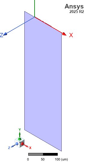
Q2D Cross-Section Geometry#
Here is the 2D geometry of the CPW cross-section in Ansys 2D Extractor.
# Ensure Q2D model fits the screen
q2d.modeler.fit_all()

# Save screenshot
img_dir = PATH.repo / "docs" / "_static" / "images"
img_dir.mkdir(parents=True, exist_ok=True)
q2d_img_path = img_dir / "q2d_cpw_impedance_geom.jpg"
q2d.post.export_model_picture(
    full_name=str(q2d_img_path), show_axis=True, show_grid=False, show_ruler=True
)

# Display in notebook
display(Image(filename=str(q2d_img_path)))
PyAEDT INFO: Parsing /tmp/tmp70dmm41z.ansys_qpdk/cpw_q2d.aedt.
PyAEDT INFO: File /tmp/tmp70dmm41z.ansys_qpdk/cpw_q2d.aedt correctly loaded. Elapsed time: 0m 0sec
PyAEDT INFO: aedt file load time 0.002233743667602539
PyAEDT INFO: PostProcessor class has been initialized! Elapsed time: 0m 0sec
PyAEDT INFO: Post class has been initialized! Elapsed time: 0m 0sec

Configure Q2D Analysis#
Set up the solution with a frequency sweep from 1 GHz to 10 GHz to compute the characteristic impedance across the frequency range.
# Create setup
setup = q2d.create_setup(name="Q2DSetup")

# Add frequency sweep
sweep = setup.add_sweep(name="FrequencySweep")
sweep.props["RangeType"] = "LinearStep"
sweep.props["RangeStart"] = f"{Q2D_CONFIG['sweep_start_ghz']}GHz"
sweep.props["RangeStep"] = f"{Q2D_CONFIG['sweep_step_ghz']}GHz"
sweep.props["RangeEnd"] = f"{Q2D_CONFIG['sweep_stop_ghz']}GHz"
sweep.props["Type"] = "Interpolating"
sweep.update()

print("Q2D setup configured:")
print(
    f"  - Sweep range: {Q2D_CONFIG['sweep_start_ghz']} – {Q2D_CONFIG['sweep_stop_ghz']} GHz"
)
print(f"  - Step size: {Q2D_CONFIG['sweep_step_ghz']} GHz")
Q2D setup configured:
  - Sweep range: 1.0 – 10.0 GHz
  - Step size: 0.1 GHz
Run Simulation#
Execute the Q2D analysis.
print("Starting Q2D analysis...")
print("(This may take a few minutes)")

# Save project before analysis
q2d.save_project()

# Run the analysis
start_time = time.time()
success = q2d.analyze(cores=4)
elapsed = time.time() - start_time

if not success:
    raise RuntimeError("Q2D simulation failed. Check the AEDT log for details.")
else:
    print(f"Analysis completed in {elapsed:.1f} seconds")
Starting Q2D analysis...
(This may take a few minutes)
PyAEDT INFO: Project cpw_q2d Saved correctly
PyAEDT INFO: Project cpw_q2d Saved correctly
PyAEDT INFO: Key Desktop/ActiveDSOConfigurations/2D Extractor correctly changed.
PyAEDT INFO: Solving all design setups. Analysis started...
PyAEDT INFO: Design setup None solved correctly in 0.0h 0.0m 8.0s
PyAEDT INFO: Key Desktop/ActiveDSOConfigurations/2D Extractor correctly changed.
Analysis completed in 8.4 seconds
Extract and Plot Impedance#
Extract the characteristic impedance :math:Z_0 from Q2D and compare it
with the analytical conformal-mapping estimate. The analytical value is
shown as a horizontal dashed line.
# Extract Z0 from Q2D
data = q2d.post.get_solution_data(
    expressions="Z0(signal,signal)",
    context="Original",
    setup_sweep_name="Q2DSetup : FrequencySweep",
)

frequencies_ghz = np.array(data.primary_sweep_values)
z0_q2d = np.array(data.data_real())

# --- Plot ---
fig, ax = plt.subplots(figsize=(10, 5))

# Q2D result
ax.plot(frequencies_ghz, z0_q2d, "b-", linewidth=2, label="Q2D (quasi-static)")

# Analytical estimate as a horizontal line
ax.axhline(
    y=z0_analytical,
    color="r",
    linestyle="--",
    linewidth=1.5,
    label=f"Analytical (conformal mapping): {z0_analytical:.2f} Ω",
)

ax.set_xlabel("Frequency (GHz)")
ax.set_ylabel("Characteristic Impedance $Z_0$ (Ω)")
ax.set_title("CPW Characteristic Impedance: Q2D vs. Analytical Estimate")
ax.legend()
ax.grid(True)
ax.set_xlim(Q2D_CONFIG["sweep_start_ghz"], Q2D_CONFIG["sweep_stop_ghz"])

plt.tight_layout()
plt.show()

# --- Numerical comparison ---
z0_mean_q2d = np.mean(z0_q2d)
relative_diff = (z0_mean_q2d - z0_analytical) / z0_analytical * 100

print("\n=== Impedance Comparison ===")
print("-" * 45)
print(f"Analytical Z₀ (conformal mapping): {z0_analytical:.2f} Ω")
print(f"Q2D Z₀ (mean over frequency):      {z0_mean_q2d:.2f} Ω")
print(f"Relative difference:                {relative_diff:+.2f}%")
print("-" * 45)
PyAEDT WARNING: No report category provided. Automatically identified Matrix
PyAEDT INFO: Solution Correctly loaded. Elapsed time: 0m 0sec
PyAEDT INFO: Solution Correctly parsed. Elapsed time: 0m 0sec
~/dev/quantum-rf-pdk/.venv/lib/python3.12/site-packages/ansys/aedt/core/visualization/post/solution_data.py:648: UserWarning: Method `data_real` is deprecated. Use :func:`get_expression_data` property instead.
  warnings.warn("Method `data_real` is deprecated. Use :func:`get_expression_data` property instead.")
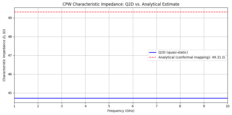
=== Impedance Comparison ===
---------------------------------------------
Analytical Z₀ (conformal mapping): 49.31 Ω
Q2D Z₀ (mean over frequency):      44.72 Ω
Relative difference:                -9.32%
---------------------------------------------
Cleanup#
Close the Q2D session and clean up temporary files.
# Save and close
q2d.save_project()
# q2d.release_desktop()  # Uncomment to close the AEDT desktop session
time.sleep(2)

# Clean up temp directory
temp_dir.cleanup()
print("Q2D session closed and temporary files cleaned up")
PyAEDT INFO: Project cpw_q2d Saved correctly
Q2D session closed and temporary files cleaned up
Summary#
This notebook demonstrated:
Cross-Section Definition: Using QPDK’s
coplanar_waveguidecross-section to define CPW geometry (10 µm width, 6 µm gap)Q2D Setup: Initializing Ansys 2D Extractor via PyAEDT and building the cross-sectional geometry using :meth:
~qpdk.simulation.q3d.Q2D.create_2d_from_cross_sectionImpedance Extraction: Running the Q2D quasi-static solver to compute :math:
Z_0as a function of frequency from 1 to 10 GHzAnalytical Validation: Comparing the Q2D result with the conformal-mapping analytical estimate from :func:
~qpdk.models.cpw.cpw_parameters
Key Points for CPW Design:
The Q2D solver gives frequency-dependent impedance including dispersion effects
The analytical conformal-mapping model provides a good quasi-static estimate
For superconducting CPWs (PEC conductors), the impedance is nearly frequency-independent in the low-GHz range
No backplate metallisation is used, matching typical superconducting fabrication
Next Steps:
Vary CPW dimensions to study impedance sensitivity
Compare with HFSS 3D driven-modal simulations
Study the effect of conductor thickness on impedance
References#
Rainee Simons. Coplanar Waveguide Circuits, Components, and Systems. Number v. 165 in Wiley Series in Microwave and Optical Engineering. Wiley Interscience, New York, 2001. ISBN 978-0-471-46393-1. doi:10.1002/0471224758.