

HFSS Driven Modal Simulation of an Interdigital Capacitor#
This notebook demonstrates how to set up and run a driven modal (S-parameter) simulation of an interdigital capacitor using PyAEDT (Ansys HFSS Python interface).
Driven modal analysis computes scattering parameters (S-parameters) of structures with ports, enabling characterization of coupling capacitance, insertion loss, and frequency-dependent behavior.
Prerequisites:
Ansys HFSS installed (requires license)
Install hfss extras:
uv sync --extra hfssorpip install qpdk[hfss]
References:
PyAEDT Documentation: https://aedt.docs.pyansys.com/
HFSS Driven Modal Examples: https://examples.aedt.docs.pyansys.com/
Interdigital Capacitor Theory: [LeiZhuW00]
Setup and Imports#
Estimate Capacitance#
Before running the full-wave simulation, we can estimate the mutual capacitance using the analytical conformal mapping model for interdigital capacitors [ID04].
For a structure with \(n\) fingers of width \(w\), gap \(g\), and overlap length \(L\), the metallization ratio is \(\eta = \frac{w}{w + g}\). The interior and exterior capacitances per unit length are derived using the complete elliptic integrals of the first kind \(K(k)\):
The total mutual capacitance for \(n\) fingers is then:
# Get substrate permittivity from cross-section
ep_r = cpw_ep_r_from_cross_section(cross_section)

# Analytical estimate using QPDK model
C_estimate = interdigital_capacitor_capacitance_analytical(
    fingers=6,
    finger_length=20.0,
    finger_gap=2.0,
    thickness=5.0,
    ep_r=float(ep_r),
)
print(f"Estimated capacitance: {float(C_estimate) * 1e15:.2f} fF")
Estimated capacitance: 8.19 fF
Initialize HFSS Project#
Set up an HFSS project for driven modal analysis with ports.
Note: This section requires Ansys HFSS to be installed and licensed.
# Configuration for HFSS simulation
HFSS_CONFIG = {
    "solution_frequency_ghz": 5.0,  # Adaptive mesh at 5 GHz
    "sweep_start_ghz": 0.1,  # Sweep from 100 MHz
    "sweep_stop_ghz": 20.0,  # to 20 GHz
    "sweep_points": 401,  # Number of frequency points
    "max_passes": 16,
    "max_delta_s": 0.002,  # 0.2% S-parameter convergence
}
Build HFSS Model (Example Code)#
The following demonstrates the complete workflow for driven modal simulation:
Create HFSS project with “DrivenModal” solution type
Build capacitor geometry with ports
Configure frequency sweep
Run simulation and extract S-parameters
Note
This code requires Ansys HFSS. The structure below shows the complete workflow.
# Example HFSS driven modal simulation workflow
# This code block demonstrates the full workflow but requires HFSS license

# Ensure Ansys path is set so PyAEDT can find it
ansys_default_path = "/usr/ansys_inc/v252/AnsysEM"
if "ANSYSEM_ROOT252" not in os.environ and Path(ansys_default_path).exists():
    os.environ["ANSYSEM_ROOT252"] = ansys_default_path

settings.use_grpc_uds = False


# Create temporary directory for project
temp_dir = tempfile.TemporaryDirectory(suffix=".ansys_qpdk")
project_path = Path(temp_dir.name) / "idc_driven.aedt"

# Initialize HFSS with Driven Modal solution
hfss = Hfss(
    project=str(project_path),
    design="InterdigitalCapacitor",
    solution_type="DrivenModal",
    non_graphical=False,
    new_desktop=True,
    version="2025.2",
)
hfss.modeler.model_units = "um"

print(f"HFSS project created: {hfss.project_file}")
print(f"Design name: {hfss.design_name}")
print(f"Solution type: {hfss.solution_type}")
PyAEDT INFO: Python version 3.12.13 (main, Mar 3 2026, 14:59:34) [Clang 21.1.4 ].
PyAEDT INFO: PyAEDT version 0.26.2.
PyAEDT INFO: Initializing new Desktop session.
PyAEDT INFO: AEDT version 2025.2.
PyAEDT INFO: New AEDT session is starting on gRPC port 54607.
PyAEDT INFO: Starting new AEDT gRPC session on port 54607.
PyAEDT INFO: Launching AEDT server with gRPC transport mode: TransportMode.UDS
PyAEDT INFO: Electronics Desktop started on gRPC port 54607 after 9.2 seconds.
PyAEDT INFO: AEDT installation Path /usr/ansys_inc/v252/AnsysEM
PyAEDT INFO: Connected to AEDT gRPC session on port 54607.
PyAEDT WARNING: Service Pack is not detected. PyAEDT is currently connecting in Insecure Mode.
PyAEDT WARNING: Please download and install latest Service Pack to use connect to AEDT in Secure Mode.
PyAEDT INFO: Project idc_driven has been created.
PyAEDT INFO: Added design 'InterdigitalCapacitor' of type HFSS.
PyAEDT INFO: AEDT objects correctly read
PyAEDT INFO: Modeler class has been initialized! Elapsed time: 0m 0sec
HFSS project created: /tmp/tmpcw93m0pr.ansys_qpdk/idc_driven.aedt
Design name: InterdigitalCapacitor
Solution type: Modal
Build Interdigital Capacitor Geometry#
Import the gdsfactory component geometry into HFSS using native GDS import.
This uses Hfss.import_gds_3d which automatically handles 3D layer mapping.
# Prepare component for export
prepared_component = prepare_component_for_aedt(idc_component, margin_draw=50)

# Initialize HFSS wrapper
hfss_sim = HFSS(hfss)

# Import the component geometry using native GDS import
success = hfss_sim.import_component(prepared_component, import_as_sheets=True)
print(f"GDS import successful: {success}")

# Add substrate below the component
substrate_name = hfss_sim.add_substrate(
    prepared_component,
    thickness=500.0,
    material="silicon",
)
print(f"Created substrate: {substrate_name}")

# Add air region for driven simulation
air_region_name = hfss_sim.add_air_region(
    prepared_component,
    height=500.0,
    substrate_thickness=500.0,
    pec_boundary=False,
)
print(f"Created air region: {air_region_name}")

# Assign radiation boundary to outer faces for driven analysis
hfss.assign_radiation_boundary_to_objects(air_region_name)
print("Assigned radiation boundary to air region")
PyAEDT INFO: GDS layer imported with elevations and thickness.
PyAEDT INFO: Boundary Perfect E PEC_Sheets has been created.
GDS import successful: True
PyAEDT INFO: Materials class has been initialized! Elapsed time: 0m 0sec
Created substrate: Substrate
Created air region: AirRegion
PyAEDT INFO: Boundary Radiation Rad__Q0YHW6 has been created.
Assigned radiation boundary to air region
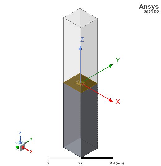
Geometry Verification#
Here is the 3D geometry of the interdigital capacitor, ready for simulation in HFSS.
# Ensure HFSS model fits the screen
hfss.modeler.fit_all()

# Save screenshot
img_dir = PATH.repo / "docs" / "_static" / "images"
img_dir.mkdir(parents=True, exist_ok=True)
hfss_img_path = img_dir / "hfss_driven_capacitor_geom.jpg"
hfss.post.export_model_picture(
    full_name=str(hfss_img_path), show_axis=True, show_grid=False, show_ruler=True
)

# Display in notebook
display(Image(filename=str(hfss_img_path)))
PyAEDT INFO: Parsing /tmp/tmpcw93m0pr.ansys_qpdk/idc_driven.aedt.
PyAEDT INFO: File /tmp/tmpcw93m0pr.ansys_qpdk/idc_driven.aedt correctly loaded. Elapsed time: 0m 0sec
PyAEDT INFO: aedt file load time 0.0027740001678466797
PyAEDT INFO: PostProcessor class has been initialized! Elapsed time: 0m 0sec
PyAEDT INFO: PostProcessor class has been initialized! Elapsed time: 0m 0sec
PyAEDT INFO: Post class has been initialized! Elapsed time: 0m 0sec

Create Lumped Ports#
Add lumped ports at both ends of the capacitor to measure S-parameters. The ports are placed at the CPW feed locations.
print("Creating lumped ports.")

hfss_sim.add_lumped_ports(prepared_component.ports, cpw_gap, cpw_width)
for port in prepared_component.ports:
    print(
        f"  Created {port.name} at {port.center} with orientation {port.orientation}°"
    )
Creating lumped ports.
PyAEDT INFO: Boundary Lumped Port o1 has been created.
PyAEDT INFO: Boundary Lumped Port o2 has been created.
  Created o1 at (-23.0, 0.0) with orientation 180.0°
  Created o2 at (23.0, 0.0) with orientation 0.0°
Configure Driven Modal Analysis#
Set up the solution with frequency sweep to compute S-parameters across the desired frequency range.
# Create driven modal setup
setup = hfss.create_setup(
    name="DrivenSetup",
    Frequency=f"{HFSS_CONFIG['solution_frequency_ghz']}GHz",
)

setup.props["MaxDeltaS"] = HFSS_CONFIG["max_delta_s"]
setup.props["MaximumPasses"] = HFSS_CONFIG["max_passes"]
setup.props["MinimumPasses"] = 2
setup.props["PercentRefinement"] = 30
setup.update()

# Create frequency sweep
sweep = setup.create_frequency_sweep(
    unit="GHz",
    name="FrequencySweep",
    start_frequency=HFSS_CONFIG["sweep_start_ghz"],
    stop_frequency=HFSS_CONFIG["sweep_stop_ghz"],
    sweep_type="Interpolating",
    num_of_freq_points=HFSS_CONFIG["sweep_points"],
)

print("Driven modal setup configured:")
print(f"  - Solution frequency: {HFSS_CONFIG['solution_frequency_ghz']} GHz")
print(
    f"  - Sweep range: {HFSS_CONFIG['sweep_start_ghz']} - {HFSS_CONFIG['sweep_stop_ghz']} GHz"
)
print(f"  - Number of points: {HFSS_CONFIG['sweep_points']}")
PyAEDT INFO: Linear count sweep FrequencySweep has been correctly created
Driven modal setup configured:
  - Solution frequency: 5.0 GHz
  - Sweep range: 0.1 - 20.0 GHz
  - Number of points: 401
Run Simulation#
Execute the driven modal analysis with frequency sweep.
print("Starting driven modal analysis...")
print("(This may take several minutes)")

# Save project before analysis
hfss.save_project()

# Run the analysis
start_time = time.time()
success = hfss.analyze_setup("DrivenSetup", cores=4)
elapsed = time.time() - start_time

if not success:
    print("\nERROR: HFSS simulation failed!")
else:
    print(f"Analysis completed in {elapsed:.1f} seconds")
Starting driven modal analysis...
(This may take several minutes)
PyAEDT INFO: Project idc_driven Saved correctly
PyAEDT INFO: Key Desktop/ActiveDSOConfigurations/HFSS correctly changed.
PyAEDT INFO: Solving design setup DrivenSetup
PyAEDT INFO: Design setup DrivenSetup solved correctly in 0.0h 1.0m 21.0s
PyAEDT INFO: Key Desktop/ActiveDSOConfigurations/HFSS correctly changed.
Analysis completed in 80.8 seconds
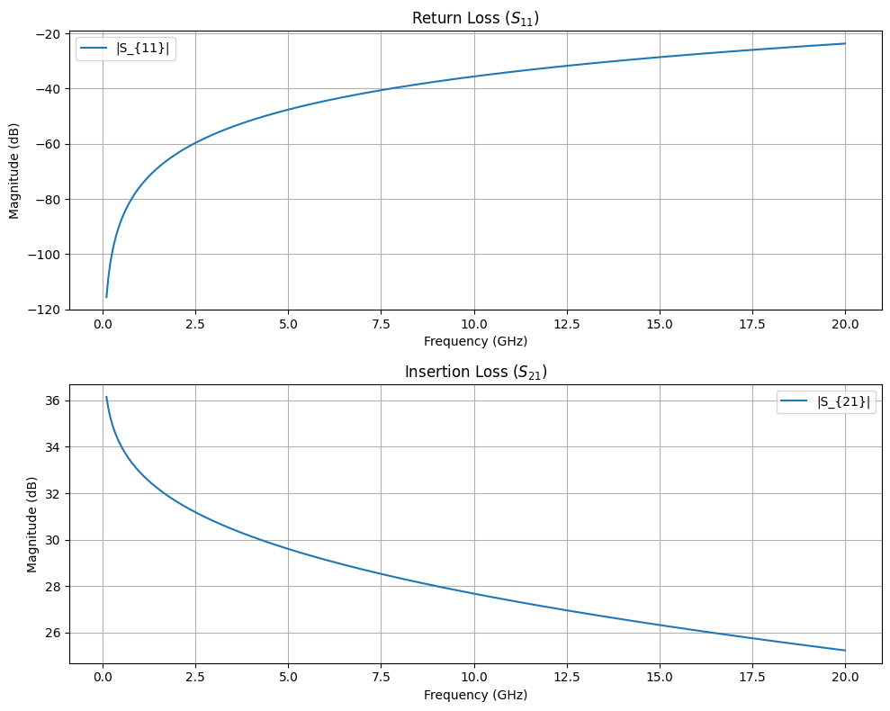
Extract and Plot S-Parameters#
Get the S-parameters from the simulation and visualize the results.
# Extract results using the wrapper
df_results = hfss_sim.get_sparameter_results(setup.name, sweep.name)

frequencies_ghz = df_results["frequency_ghz"].to_numpy()

# Plot S-parameters
fig, axes = plt.subplots(2, 1, figsize=(10, 8))

# Filter for S11 and S21 type traces
s11_col = next(col for col in df_results.columns if "S(o1:1,o1:1)" in col)
s21_col = next(col for col in df_results.columns if "S(o2:1,o1:1)" in col)

s11_trace = df_results[s11_col].to_numpy().astype(np.complex128)
s21_trace = df_results[s21_col].to_numpy().astype(np.complex128)

s11_mag_db = 20 * np.log10(np.abs(s11_trace))
s21_mag_db = 20 * np.log10(np.abs(s21_trace))

axes[0].plot(frequencies_ghz, s11_mag_db, label=r"|S_{11}|")
axes[1].plot(frequencies_ghz, s21_mag_db, label=r"|S_{21}|")

axes[0].set_xlabel("Frequency (GHz)")
axes[0].set_ylabel("Magnitude (dB)")
axes[0].set_title("Return Loss ($S_{11}$)")
axes[0].grid(True)
axes[0].legend()

axes[1].set_xlabel("Frequency (GHz)")
axes[1].set_ylabel("Magnitude (dB)")
axes[1].set_title("Insertion Loss ($S_{21}$)")
axes[1].grid(True)
axes[1].legend()

plt.tight_layout()
# plt.show()
PyAEDT INFO: Solution Correctly loaded. Elapsed time: 0m 0sec
PyAEDT INFO: Solution Correctly parsed. Elapsed time: 0m 0sec
PyAEDT INFO: Solution Correctly loaded. Elapsed time: 0m 0sec
PyAEDT INFO: Solution Correctly parsed. Elapsed time: 0m 0sec
PyAEDT INFO: Solution Correctly loaded. Elapsed time: 0m 0sec
PyAEDT INFO: Solution Correctly parsed. Elapsed time: 0m 0sec
PyAEDT INFO: Solution Correctly loaded. Elapsed time: 0m 0sec
PyAEDT INFO: Solution Correctly parsed. Elapsed time: 0m 0sec
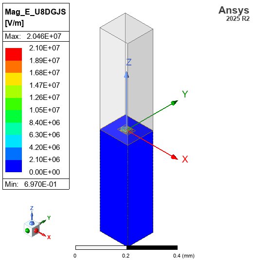
Plot Field Solution#
We can visualize the electric field magnitude on the surface of the substrate to see the capacitive coupling between the interdigital fingers.

# Ensure the model fits the screen
hfss.modeler.fit_all()

# Create a surface field plot of the electric field magnitude on the substrate
plot = hfss.post.create_fieldplot_surface(
    assignment=[substrate_name], quantity="Mag_E", setup=f"{setup.name} : LastAdaptive"
)

# Export the field plot picture
hfss_field_img_path = img_dir / "hfss_driven_capacitor_field.jpg"
if plot:
    hfss.post.export_model_picture(
        full_name=str(hfss_field_img_path),
        show_axis=True,
        show_grid=False,
        show_ruler=True,
        field_selections="all",
    )
else:
    print("Failed to create field plot")

# Display in notebook
display(Image(filename=str(hfss_field_img_path)))
PyAEDT INFO: Active Design set to InterdigitalCapacitor
Extract Capacitance from Admittance (Y-Parameters)#
Relying only on the magnitude of \(S_{21}\) assumes the geometry behaves identically to a single perfect capacitor floating in a vacuum. In reality, the structure has shunt parasitic capacitances to ground (\(C_{11}\) and \(C_{22}\)) that skew the \(S_{21}\) magnitude.
The robust way to extract mutual capacitance is using Y-parameters (Admittance), see [MP12]. In a Pi-network model, the mutual admittance \(Y_{12}\) isolates the series element:
Therefore, the exact mutual capacitance is:
# Extract Y21 parameter manually using PyAEDT's solution data
solution_y = hfss.post.get_solution_data(
    expressions="Y(o2:1,o1:1)", setup_sweep_name=f"{setup.name} : {sweep.name}"
)

# Parse complex Y-parameters
_, y_real = solution_y.get_expression_data(formula="real")
_, y_imag = solution_y.get_expression_data(formula="imag")
y21_trace = np.array(y_real) + 1j * np.array(y_imag)
frequencies_ghz_y = np.array(solution_y.primary_sweep_values)

# Analysis frequencies in GHz
analysis_frequencies_ghz = [1, 5, 10]

print("\n=== HFSS Capacitance Analysis ===")
print("-" * 40)
print(f"Analytical estimate: {C_estimate * 1e15:.2f} fF")
print("-" * 40)

C_hfss_values = {}
for freq_target in analysis_frequencies_ghz:
    idx = np.argmin(np.abs(frequencies_ghz_y - freq_target))
    freq_hz = frequencies_ghz_y[idx] * 1e9
    y21 = y21_trace[idx]

    ω = 2 * np.pi * freq_hz
    C_extracted = -np.imag(y21) / ω
    C_hfss_values[freq_target] = C_extracted

    print(
        f"At {freq_hz / 1e9:.2f} GHz: Y21 = {y21:.2e}, C ≈ {C_extracted * 1e15:.2f} fF"
    )
    print(
        f"Relative difference: {(float(C_estimate) - C_extracted) / float(C_estimate) * 100:.2f}%"
    )
PyAEDT INFO: Solution Correctly loaded. Elapsed time: 0m 0sec
PyAEDT INFO: Solution Correctly parsed. Elapsed time: 0m 0sec
=== HFSS Capacitance Analysis ===
----------------------------------------
Analytical estimate: 8.19 fF
----------------------------------------
At 1.00 GHz: Y21 = 5.76e-10-6.15e-05j, C ≈ 9.84 fF
Relative difference: -20.19%
At 4.98 GHz: Y21 = 1.43e-08-3.08e-04j, C ≈ 9.84 fF
Relative difference: -20.23%
At 10.00 GHz: Y21 = 5.73e-08-6.19e-04j, C ≈ 9.85 fF
Relative difference: -20.38%
HFSS Cleanup#
Close HFSS and clean up temporary files before starting Q3D.
# Save and close HFSS
hfss.save_project()
# hfss.release_desktop()
time.sleep(2)

# Clean up temp directory
temp_dir.cleanup()
print("HFSS session closed and temporary files cleaned up")
PyAEDT INFO: Project idc_driven Saved correctly
HFSS session closed and temporary files cleaned up
Q3D Extractor Capacitance Extraction#
Now we simulate the same geometry using Q3D Extractor, which solves quasi-static electric fields to directly compute the capacitance matrix.
Comparison of approaches:
HFSS Driven Modal: Full-wave solve → S-parameters → Y-parameters → \(C_{12}\)
Q3D Extractor: Quasi-static solve → direct capacitance matrix
Analytical: Conformal mapping model (no simulation)
Q3D is particularly well suited for parasitic capacitance extraction because it directly solves the electrostatic (or quasi-static) problem, which is faster and more accurate at low frequencies than extracting capacitance from full-wave S-parameters.
References:
Q3D Extractor: https://aedt.docs.pyansys.com/version/stable/API/_autosummary/ansys.aedt.core.q3d.Q3d.html
Initialize Q3D Project#
Set up a Q3D Extractor project for capacitance extraction.
Note
This code requires an Ansys AEDT license (same as HFSS above).
# Create temporary directory for Q3D project
temp_dir_q3d = tempfile.TemporaryDirectory(suffix=".ansys_qpdk_q3d")
project_path_q3d = Path(temp_dir_q3d.name) / "idc_q3d.aedt"

# Initialize Q3D Extractor
q3d = Q3d(
    project=str(project_path_q3d),
    design="InterdigitalCapacitor_Q3D",
    non_graphical=False,
    new_desktop=True,
    version="2025.2",
)
q3d.modeler.model_units = "um"

# Initialize Q3D wrapper
q3d_sim = Q3D(q3d)

print(f"Q3D project created: {q3d.project_file}")
print(f"Design name: {q3d.design_name}")
print(f"Solution type: {q3d.solution_type}")
PyAEDT INFO: Python version 3.12.13 (main, Mar 3 2026, 14:59:34) [Clang 21.1.4 ].
PyAEDT INFO: PyAEDT version 0.26.2.
PyAEDT INFO: Returning found Desktop session with PID 118106!
PyAEDT INFO: Project idc_q3d has been created.
PyAEDT INFO: Added design 'InterdigitalCapacitor_Q3D' of type Q3D Extractor.
PyAEDT INFO: AEDT objects correctly read
PyAEDT INFO: Modeler class has been initialized! Elapsed time: 0m 0sec
Q3D project created: /tmp/tmp_vdfv0r7.ansys_qpdk_q3d/idc_q3d.aedt
Design name: InterdigitalCapacitor_Q3D
Solution type: Q3D Extractor
Import Geometry and Assign Signal Nets#
Import the same prepared component into Q3D and assign signal nets based on port locations. Each port becomes a separate conductor in the capacitance matrix.
The q3d_sim.assign_nets_from_ports method is the Q3D equivalent
of hfss_sim.add_lumped_ports — it maps gdsfactory port locations to
Q3D conductor nets.
# Import the prepared component geometry into Q3D
conductor_objects = q3d_sim.import_component(prepared_component)
print(f"Imported {len(conductor_objects)} conductor objects: {conductor_objects}")

# Add substrate below the component (Q3D modeler API is compatible with HFSS)
substrate_q3d_name = q3d_sim.add_substrate(
    prepared_component,
    thickness=500.0,
    material="silicon",
)
print(f"Created substrate: {substrate_q3d_name}")
PyAEDT INFO: GDS layer imported with elevations and thickness.
PyAEDT INFO: Materials class has been initialized! Elapsed time: 0m 0sec
Imported 7 conductor objects: ['M1_4', 'M1_3', 'M1_6', 'M1_7', 'M1_5', 'M1_1', 'M1_2']
Created substrate: Substrate
# Assign signal nets from port locations
signal_nets = q3d_sim.assign_nets_from_ports(
    prepared_component.ports, conductor_objects
)
print(f"Assigned signal nets: {signal_nets}")
PyAEDT INFO: 3 Nets have been identified: M1_1, M1_3, M1_4
Assigned signal nets: ['o1', 'o2']
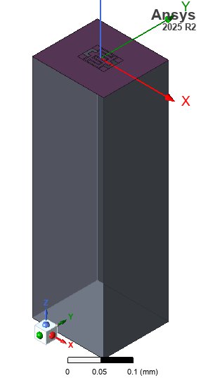
Q3D Geometry Verification#
Here is the 3D geometry of the interdigital capacitor in Q3D Extractor.
# Ensure Q3D model fits the screen
q3d.modeler.fit_all()

# Save screenshot
img_dir = PATH.repo / "docs" / "_static" / "images"
img_dir.mkdir(parents=True, exist_ok=True)
q3d_img_path = img_dir / "q3d_driven_capacitor_geom.jpg"
q3d.post.export_model_picture(
    full_name=str(q3d_img_path), show_axis=True, show_grid=False, show_ruler=True
)

# Display in notebook
display(Image(filename=str(q3d_img_path)))
PyAEDT INFO: Parsing /tmp/tmp_vdfv0r7.ansys_qpdk_q3d/idc_q3d.aedt.
PyAEDT INFO: File /tmp/tmp_vdfv0r7.ansys_qpdk_q3d/idc_q3d.aedt correctly loaded. Elapsed time: 0m 0sec
PyAEDT INFO: aedt file load time 0.002794027328491211
PyAEDT INFO: PostProcessor class has been initialized! Elapsed time: 0m 0sec
PyAEDT INFO: Post class has been initialized! Elapsed time: 0m 0sec

Configure and Run Q3D Analysis#
Set up a Q3D adaptive analysis at the same frequency used for HFSS. Q3D solves the quasi-static field problem and computes the full capacitance matrix between all signal nets.
# Create Q3D setup
q3d_setup = q3d.create_setup(name="Q3DSetup")
q3d_setup.props["AdaptiveFreq"] = f"{HFSS_CONFIG['solution_frequency_ghz']}GHz"
q3d_setup.props["Cap"]["MaxPass"] = 17
q3d_setup.props["Cap"]["MinPass"] = 2
q3d_setup.props["Cap"]["PerError"] = 0.5
# Disable AC and DC solving to avoid source/sink errors
q3d_setup.ac_rl_enabled = False
q3d_setup.dc_enabled = False
q3d_setup.capacitance_enabled = True
q3d_setup.update()

print("Q3D setup configured:")
print(f"  - Adaptive frequency: {HFSS_CONFIG['solution_frequency_ghz']} GHz")
Q3D setup configured:
  - Adaptive frequency: 5.0 GHz
print("Starting Q3D analysis...")
print("(This is typically faster than full-wave HFSS)")

q3d.save_project()

start_time_q3d = time.time()
success_q3d = q3d.analyze_setup("Q3DSetup", cores=4)
elapsed_q3d = time.time() - start_time_q3d

if not success_q3d:
    print("\nERROR: Q3D simulation failed!")
    m = q3d.desktop_class.odesktop.GetMessages(q3d.project_name, q3d.design_name, 0)
    for msg in m:
        print(f"Desktop Msg: {msg}")
else:
    print(f"Q3D analysis completed in {elapsed_q3d:.1f} seconds")
Starting Q3D analysis...
(This is typically faster than full-wave HFSS)
PyAEDT INFO: Project idc_q3d Saved correctly
PyAEDT INFO: Key Desktop/ActiveDSOConfigurations/Q3D Extractor correctly changed.
PyAEDT INFO: Solving design setup Q3DSetup
PyAEDT INFO: Design setup Q3DSetup solved correctly in 0.0h 1.0m 2.0s
PyAEDT INFO: Key Desktop/ActiveDSOConfigurations/Q3D Extractor correctly changed.
Q3D analysis completed in 61.7 seconds
Extract Q3D Capacitance Matrix#
Q3D directly outputs the capacitance matrix between all signal nets. The off-diagonal element \(C_{12}\) gives the mutual capacitance, which corresponds to the coupling capacitance of the interdigital capacitor.
# Extract the capacitance matrix using the wrapper
cap_df = q3d_sim.get_capacitance_matrix(setup_name="Q3DSetup")
print("Q3D Capacitance Matrix (F):")
print(cap_df)

# Extract mutual capacitance |C12| from the off-diagonal element
C_q3d = None
for col in cap_df.columns:
    # Match off-diagonal entries exactly between o1 and o2
    if col in {"C(o1,o2)", "C(o2,o1)"}:
        C_q3d = abs(float(cap_df[col][0]))
        break

if C_q3d is not None:
    print(f"\nQ3D mutual capacitance |C₁₂|: {C_q3d * 1e15:.2f} fF")
PyAEDT WARNING: No report category provided. Automatically identified Matrix
PyAEDT INFO: Solution Correctly loaded. Elapsed time: 0m 0sec
PyAEDT INFO: Solution Correctly parsed. Elapsed time: 0m 0sec
PyAEDT WARNING: No report category provided. Automatically identified Matrix
PyAEDT INFO: Solution Correctly loaded. Elapsed time: 0m 0sec
PyAEDT INFO: Solution Correctly parsed. Elapsed time: 0m 0sec
PyAEDT WARNING: No report category provided. Automatically identified Matrix
PyAEDT INFO: Solution Correctly loaded. Elapsed time: 0m 0sec
PyAEDT INFO: Solution Correctly parsed. Elapsed time: 0m 0sec
PyAEDT WARNING: No report category provided. Automatically identified Matrix
PyAEDT INFO: Solution Correctly loaded. Elapsed time: 0m 0sec
PyAEDT INFO: Solution Correctly parsed. Elapsed time: 0m 0sec
PyAEDT WARNING: No report category provided. Automatically identified Matrix
~/dev/quantum-rf-pdk/.venv/lib/python3.12/site-packages/ansys/aedt/core/visualization/post/solution_data.py:648: UserWarning: Method `data_real` is deprecated. Use :func:`get_expression_data` property instead.
  warnings.warn("Method `data_real` is deprecated. Use :func:`get_expression_data` property instead.")
PyAEDT INFO: Solution Correctly loaded. Elapsed time: 0m 0sec
PyAEDT INFO: Solution Correctly parsed. Elapsed time: 0m 0sec
PyAEDT WARNING: No report category provided. Automatically identified Matrix
PyAEDT INFO: Solution Correctly loaded. Elapsed time: 0m 0sec
PyAEDT INFO: Solution Correctly parsed. Elapsed time: 0m 0sec
Q3D Capacitance Matrix (F):
shape: (1, 6)
┌──────────────┬─────────────┬─────────────┬────────────┬─────────────┬────────────┐
│ C(M1_1,M1_1) ┆ C(M1_1,o1)  ┆ C(M1_1,o2)  ┆ C(o1,o1)   ┆ C(o1,o2)    ┆ C(o2,o2)   │
│ ---          ┆ ---         ┆ ---         ┆ ---        ┆ ---         ┆ ---        │
│ f64          ┆ f64         ┆ f64         ┆ f64        ┆ f64         ┆ f64        │
╞══════════════╪═════════════╪═════════════╪════════════╪═════════════╪════════════╡
│ 2.8507e-14   ┆ -9.2535e-15 ┆ -9.2194e-15 ┆ 1.8289e-14 ┆ -8.7666e-15 ┆ 1.8264e-14 │
└──────────────┴─────────────┴─────────────┴────────────┴─────────────┴────────────┘

Q3D mutual capacitance |C₁₂|: 8.77 fF
Q3D Cleanup#
q3d.save_project()
# q3d.release_desktop()
time.sleep(2)

temp_dir_q3d.cleanup()
print("Q3D session closed and temporary files cleaned up")
PyAEDT INFO: Project idc_q3d Saved correctly
Q3D session closed and temporary files cleaned up
Comparison: Analytical vs HFSS vs Q3D#
Compare the capacitance values obtained from all three methods. The analytical model provides a quick estimate, the HFSS driven modal simulation gives the full-wave result, and Q3D Extractor provides a direct quasi-static capacitance extraction.
print("\n" + "=" * 58)
print("          Capacitance Comparison Summary")
print("=" * 58)
print(f"{'Method':<28} {'C (fF)':>10} {'Δ vs Analytical':>16}")
print("-" * 58)

C_analytical_fF = float(C_estimate) * 1e15
print(f"{'Analytical':<28} {C_analytical_fF:>10.2f} {'(reference)':>16}")

for freq_ghz, c_val in C_hfss_values.items():
    c_fF = c_val * 1e15
    delta = (c_val - float(C_estimate)) / float(C_estimate) * 100
    label = f"HFSS @ {freq_ghz} GHz"
    print(f"{label:<28} {c_fF:>10.2f} {delta:>+15.1f}%")

if C_q3d is not None:
    C_q3d_fF = C_q3d * 1e15
    delta_q3d = (C_q3d - float(C_estimate)) / float(C_estimate) * 100
    print(f"{'Q3D Extractor':<28} {C_q3d_fF:>10.2f} {delta_q3d:>+15.1f}%")

print("=" * 58)
==========================================================
          Capacitance Comparison Summary
==========================================================
Method                           C (fF)  Δ vs Analytical
----------------------------------------------------------
Analytical                         8.19      (reference)
HFSS @ 1 GHz                       9.84           +20.2%
HFSS @ 5 GHz                       9.84           +20.2%
HFSS @ 10 GHz                      9.85           +20.4%
Q3D Extractor                      8.77            +7.1%
==========================================================
Summary#
This notebook demonstrated three approaches for characterizing an interdigital capacitor:
Analytical Estimate: Using the conformal mapping model for interdigital capacitors to get a quick capacitance estimate without simulation
HFSS Driven Modal Simulation:
Created the component geometry with QPDK and imported it into HFSS
Added lumped ports at CPW feed locations for S-parameter measurements
Ran a frequency sweep and extracted capacitance from Y-parameters (\(C_{12} = -\text{Im}(Y_{12}) / \omega\))
Q3D Extractor Simulation:
Imported the same geometry into Q3D Extractor
Assigned signal nets from gdsfactory port locations
Directly computed the capacitance matrix via quasi-static field solution
Key Takeaways:
Q3D Extractor directly solves for capacitance, making it ideal for parasitic extraction at low frequencies
HFSS driven modal captures frequency-dependent effects (parasitic inductance, radiation) that Q3D’s quasi-static approach does not
The analytical model provides a useful sanity check for both simulations
All three methods should agree well at low frequencies where the structure is electrically small
References#
Rui Igreja and C. J. Dias. Analytical evaluation of the interdigital electrodes capacitance for a multi-layered structure. Sensors and Actuators A: Physical, 112(2):291–301, May 2004. doi:10.1016/j.sna.2004.01.040.
David M. Pozar. Microwave Engineering. John Wiley & Sons, Inc., 4 edition, 2012. ISBN 978-0-470-63155-3.
Lei Zhu and Ke Wu. Accurate circuit model of interdigital capacitor and its application to design of new quasi-lumped miniaturized filters with suppression of harmonic resonance. IEEE Transactions on Microwave Theory and Techniques, 48(3):347–356, March 2000. doi:10.1109/22.826833.