Circuit simulations (tidy3d + SAX)

Sparameters are common in RF and photonic simulation.

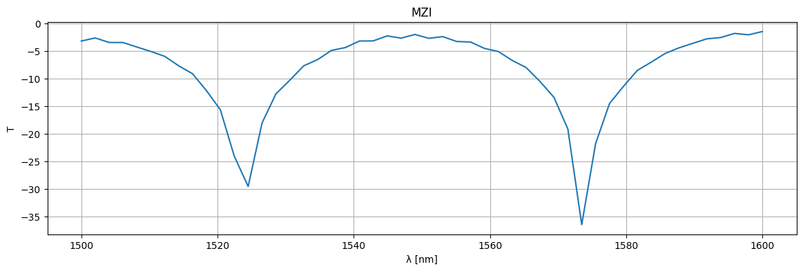
We are going to simulate a MZI interferometer circuit.

For that we need to simulate each of the component Sparameters in tidy3d and then SAX Sparameter circuit solver to solve the Sparameters for the circuit.

We will be using SAX which is open source and tidy3d which requires you to create an account to run simulations in tidy3d cloud.

tidy3d FDTD simulations

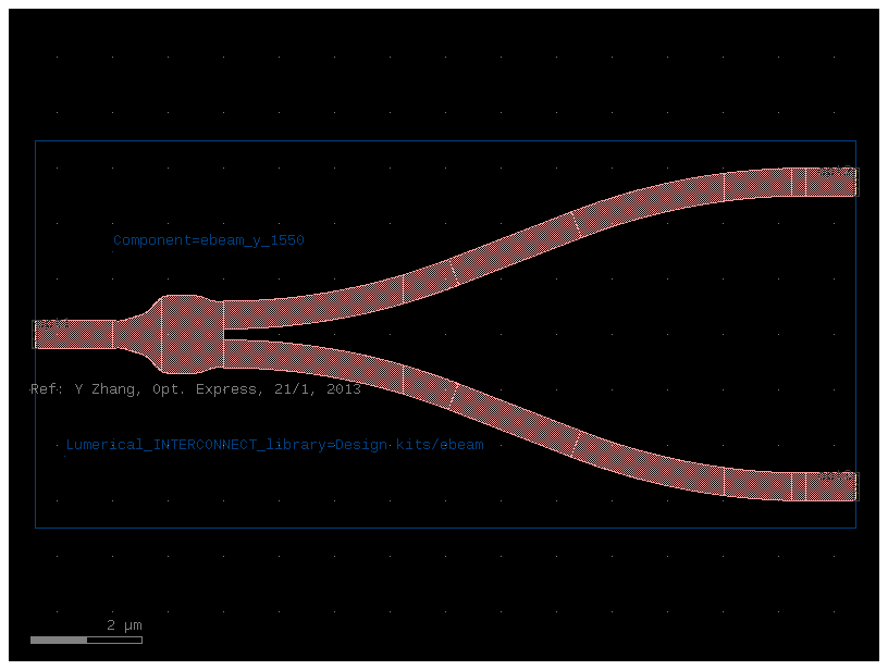
Lets compute the Sparameters of a 1x2 power splitter using tidy3d.

tidy3D is a fast GPU based FDTD tool developed by flexcompute.

To run, you need to create an account and add credits. The number of credits that each simulation takes depends on the simulation computation time.

import gplugins as sim
import gplugins.tidy3d as gt

import ubcpdk.components as pdk
from ubcpdk.config import PATH

c = pdk.ebeam_y_1550()
c.plot()

sp = gt.write_sparameters(c, filepath=PATH.sparameters / "ebeam_y_1550_20634f71.npz")

17:37:06 UTC WARNING: 'simulation.structures[0]' is outside of the simulation   
             domain.                                                            

             WARNING: 'simulation.structures[0]' is outside of the simulation   
             domain.                                                            

Simulation loaded from PosixPath('/__w/ubc/ubc/sparameters/ebeam_y_1550_20634f71.npz')

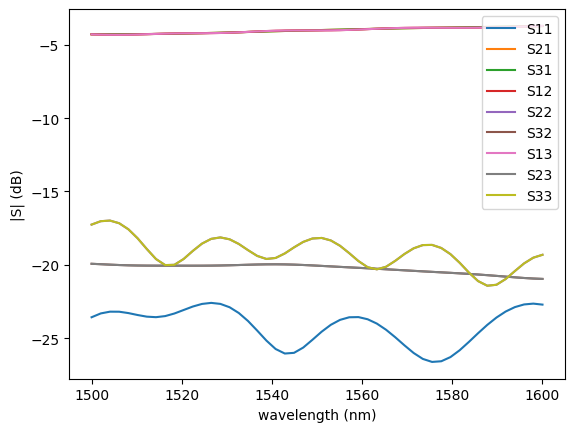
sim.plot.plot_sparameters(sp)

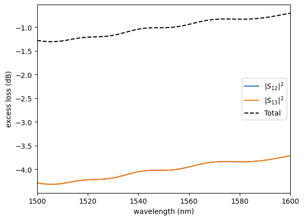
sim.plot.plot_loss1x2(sp)

Circuit simulation

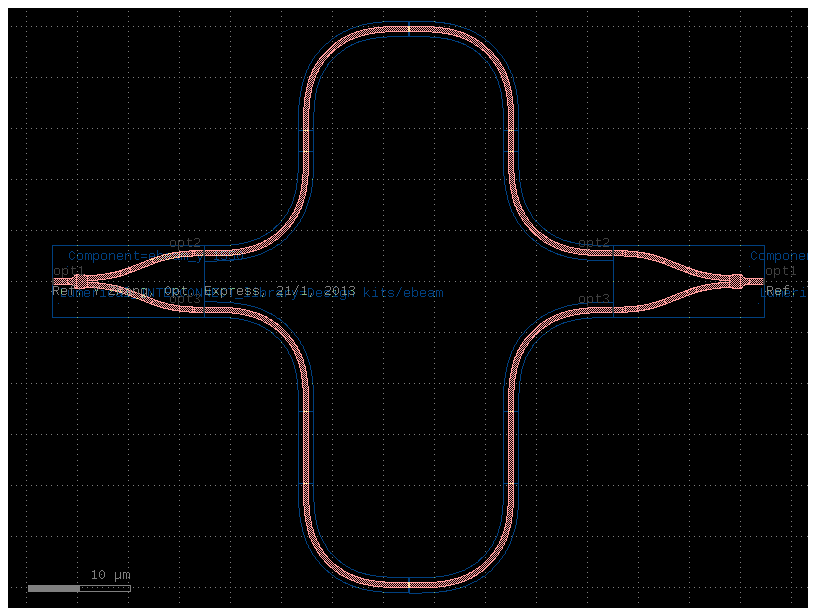
mzi10 = pdk.mzi(splitter=c, delta_length=10)
mzi10.plot()

import gplugins.sax as gsax
import jax.numpy as jnp
import matplotlib.pyplot as plt
import numpy as np
import sax

def straight(wl=1.5, length=10.0, neff=2.4) -> sax.SDict:
    return sax.reciprocal({("o1", "o2"): jnp.exp(2j * jnp.pi * neff * length / wl)})


def bend_euler(wl=1.5, length=20.0):
    """Assumes a reduced transmission for the euler bend compared to a straight"""
    return {k: 0.99 * v for k, v in straight(wl=wl, length=length).items()}

ebeam_y_1550 = gsax.read.model_from_npz(sp)

netlist = mzi10.get_netlist()
circuit, _ = sax.circuit(
    netlist=netlist,
    models={
        "bend_euler": bend_euler,
        "ebeam_y_1550": ebeam_y_1550,
        "straight": straight,
    },
)

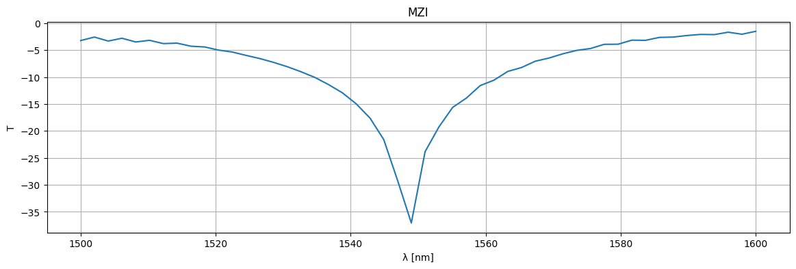
wl = np.linspace(1.5, 1.6)
S = circuit(wl=wl)
plt.figure(figsize=(14, 4))
plt.title("MZI")
plt.plot(1e3 * wl, 10 * np.log10(jnp.abs(S["o1", "o2"]) ** 2))
plt.xlabel("λ [nm]")
plt.ylabel("T")
plt.grid(True)
plt.show()

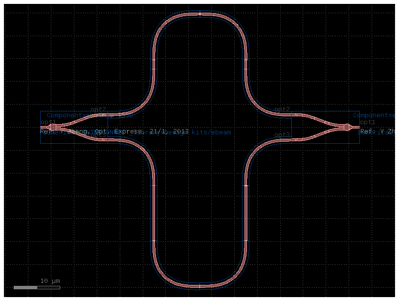
mzi20 = pdk.mzi(splitter=c, delta_length=20)
mzi20.plot()

netlist = mzi20.get_netlist()
circuit, _ = sax.circuit(
    netlist=netlist,
    models={
        "bend_euler": bend_euler,
        "ebeam_y_1550": ebeam_y_1550,
        "straight": straight,
    },
)

wl = np.linspace(1.5, 1.6)
S = circuit(wl=wl)
plt.figure(figsize=(14, 4))
plt.title("MZI")
plt.plot(1e3 * wl, 10 * np.log10(jnp.abs(S["o1", "o2"]) ** 2))
plt.xlabel("λ [nm]")
plt.ylabel("T")
plt.grid(True)
plt.show()