SAX circuit simulator#
SAX is a circuit solver written in JAX, writing your component models in SAX enables you not only to get the function values but the gradients, this is useful for circuit optimization.
This tutorial has been adapted from the SAX Quick Start.
You can install sax with pip (read the SAX install instructions here)
pip install 'gplugins[sax]'
from functools import partial
from pprint import pprint

import gdsfactory as gf
import gplugins.sax as gs
import gplugins.tidy3d as gt
import jax.numpy as jnp
import matplotlib.pyplot as plt
import numpy as np
import sax

# Activate the generic PDK for gdsfactory components
gf.gpdk.PDK.activate()
Scatter dictionaries#
The core datastructure for specifying scatter parameters in SAX is a dictionary… more specifically a dictionary which maps a port combination (2-tuple) to a scatter parameter (or an array of scatter parameters when considering multiple wavelengths for example). Such a specific dictionary mapping is called ann SDict in SAX (SDict ≈ Dict[Tuple[str,str], float]).
Dictionaries are in fact much better suited for characterizing S-parameters than, say, (jax-)numpy arrays due to the inherent sparse nature of scatter parameters. Moreover, dictionaries allow for string indexing, which makes them much more pleasant to use in this context.
o2            o3
   \        /
    ========
   /        \
o1            o4
nm = 1e-3
coupling = 0.5
kappa = coupling**0.5
tau = (1 - coupling) ** 0.5
coupler_dict = {
    ("o1", "o4"): tau,
    ("o4", "o1"): tau,
    ("o1", "o3"): 1j * kappa,
    ("o3", "o1"): 1j * kappa,
    ("o2", "o4"): 1j * kappa,
    ("o4", "o2"): 1j * kappa,
    ("o2", "o3"): tau,
    ("o3", "o2"): tau,
}
coupler_dict
{('o1', 'o4'): 0.7071067811865476,
 ('o4', 'o1'): 0.7071067811865476,
 ('o1', 'o3'): 0.7071067811865476j,
 ('o3', 'o1'): 0.7071067811865476j,
 ('o2', 'o4'): 0.7071067811865476j,
 ('o4', 'o2'): 0.7071067811865476j,
 ('o2', 'o3'): 0.7071067811865476,
 ('o3', 'o2'): 0.7071067811865476}
it can still be tedious to specify every port in the circuit manually. SAX therefore offers the reciprocal function, which auto-fills the reverse connection if the forward connection exist. For example:
coupler_dict = sax.reciprocal(
    {
        ("o1", "o4"): tau,
        ("o1", "o3"): 1j * kappa,
        ("o2", "o4"): 1j * kappa,
        ("o2", "o3"): tau,
    }
)

coupler_dict
{('o1', 'o4'): 0.7071067811865476,
 ('o1', 'o3'): 0.7071067811865476j,
 ('o2', 'o4'): 0.7071067811865476j,
 ('o2', 'o3'): 0.7071067811865476,
 ('o4', 'o1'): 0.7071067811865476,
 ('o3', 'o1'): 0.7071067811865476j,
 ('o4', 'o2'): 0.7071067811865476j,
 ('o3', 'o2'): 0.7071067811865476}
Parametrized Models#
Constructing such an SDict is easy, however, usually we’re more interested in having parametrized models for our components. To parametrize the coupler SDict, just wrap it in a function to obtain a SAX Model, which is a keyword-only function mapping to an SDict:
def coupler(coupling=0.5) -> sax.SDict:
    kappa = coupling**0.5
    tau = (1 - coupling) ** 0.5
    return sax.reciprocal(
        {
            ("o1", "o4"): tau,
            ("o1", "o3"): 1j * kappa,
            ("o2", "o4"): 1j * kappa,
            ("o2", "o3"): tau,
        }
    )


coupler(coupling=0.3)
{('o1', 'o4'): 0.8366600265340756,
 ('o1', 'o3'): 0.5477225575051661j,
 ('o2', 'o4'): 0.5477225575051661j,
 ('o2', 'o3'): 0.8366600265340756,
 ('o4', 'o1'): 0.8366600265340756,
 ('o3', 'o1'): 0.5477225575051661j,
 ('o4', 'o2'): 0.5477225575051661j,
 ('o3', 'o2'): 0.8366600265340756}
def waveguide(wl=1.55, wl0=1.55, neff=2.34, ng=3.4, length=10.0, loss=0.0) -> sax.SDict:
    dwl = wl - wl0
    dneff_dwl = (ng - neff) / wl0
    neff = neff - dwl * dneff_dwl
    phase = 2 * jnp.pi * neff * length / wl
    transmission = 10 ** (-loss * length / 20) * jnp.exp(1j * phase)
    return sax.reciprocal(
        {
            ("o1", "o2"): transmission,
        }
    )
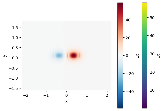
Waveguide model#
You can create a dispersive waveguide model in SAX.
Lets compute the effective index neff and group index ng for a 1550nm 500nm straight waveguide
strip = gt.modes.Waveguide(
    wavelength=1.55,
    core_width=0.5,
    core_thickness=0.22,
    slab_thickness=0.0,
    core_material="si",
    clad_material="sio2",
    group_index_step=10 * nm,
)
strip.plot_field(field_name="Ex", mode_index=0)  # TE
/home/runner/work/ubc/ubc/.venv/lib/python3.12/site-packages/tidy3d/components/mode/derivatives.py:14: FutureWarning: Input has data type int64, but the output has been cast to float64.  In the future, the output data type will match the input. To avoid this warning, set the `dtype` parameter to `None` to have the output dtype match the input, or set it to the desired output data type.
  dxf = sp.csr_matrix(sp.diags([-1, 1], [0, 1], shape=(Nx, Nx)))
/home/runner/work/ubc/ubc/.venv/lib/python3.12/site-packages/tidy3d/components/mode/derivatives.py:27: FutureWarning: Input has data type int64, but the output has been cast to float64.  In the future, the output data type will match the input. To avoid this warning, set the `dtype` parameter to `None` to have the output dtype match the input, or set it to the desired output data type.
  dxb = sp.csr_matrix(sp.diags([1, -1], [0, -1], shape=(Nx, Nx)))
/home/runner/work/ubc/ubc/.venv/lib/python3.12/site-packages/tidy3d/components/mode/derivatives.py:42: FutureWarning: Input has data type int64, but the output has been cast to float64.  In the future, the output data type will match the input. To avoid this warning, set the `dtype` parameter to `None` to have the output dtype match the input, or set it to the desired output data type.
  dyf = sp.csr_matrix(sp.diags([-1, 1], [0, 1], shape=(Ny, Ny)))
/home/runner/work/ubc/ubc/.venv/lib/python3.12/site-packages/tidy3d/components/mode/derivatives.py:55: FutureWarning: Input has data type int64, but the output has been cast to float64.  In the future, the output data type will match the input. To avoid this warning, set the `dtype` parameter to `None` to have the output dtype match the input, or set it to the desired output data type.
  dyb = sp.csr_matrix(sp.diags([1, -1], [0, -1], shape=(Ny, Ny)))
<matplotlib.collections.QuadMesh at 0x7f001ea5a030>
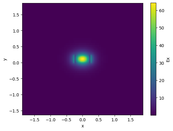
neff = strip.n_eff[0]
print(neff)
(2.5113473360975034+4.427776281277697e-05j)
ng = strip.n_group[0]
print(ng)
4.17803969357451
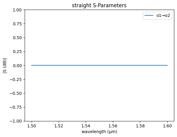
straight_sc = partial(gs.models.straight, neff=float(neff), ng=ng)
/tmp/ipykernel_2643/2582245833.py:1: ComplexWarning: Casting complex values to real discards the imaginary part
  straight_sc = partial(gs.models.straight, neff=float(neff), ng=ng)
gs.plot_model(straight_sc)
plt.ylim(-1, 1)
(-1.0, 1.0)
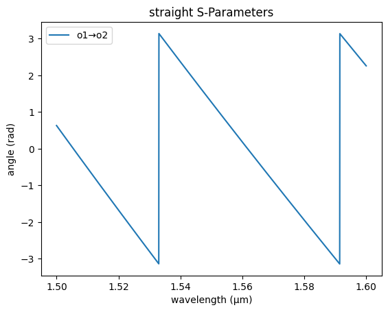
gs.plot_model(straight_sc, phase=True)
<Axes: title={'center': 'straight S-Parameters'}, xlabel='wavelength (µm)', ylabel='angle (rad)'>
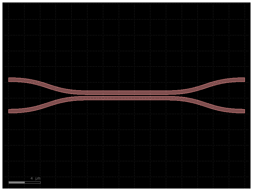
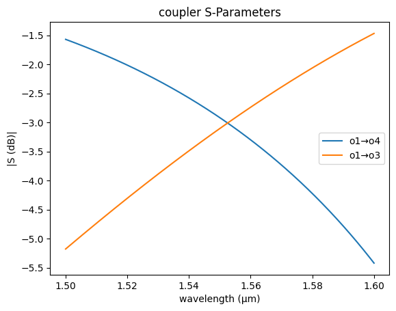
Coupler model#
Lets define the model for an evanescent coupler
c = gf.components.coupler(length=10, gap=0.2)
c.plot()
nm = 1e-3
cp = gt.modes.WaveguideCoupler(
    wavelength=1.55,
    core_width=(500 * nm, 500 * nm),
    gap=200 * nm,
    core_thickness=220 * nm,
    slab_thickness=0 * nm,
    core_material="si",
    clad_material="sio2",
)

cp.plot_field(field_name="Ex", mode_index=0)  # even mode
cp.plot_field(field_name="Ex", mode_index=1)  # odd mode
/home/runner/work/ubc/ubc/.venv/lib/python3.12/site-packages/tidy3d/components/mode/derivatives.py:14: FutureWarning: Input has data type int64, but the output has been cast to float64.  In the future, the output data type will match the input. To avoid this warning, set the `dtype` parameter to `None` to have the output dtype match the input, or set it to the desired output data type.
  dxf = sp.csr_matrix(sp.diags([-1, 1], [0, 1], shape=(Nx, Nx)))
/home/runner/work/ubc/ubc/.venv/lib/python3.12/site-packages/tidy3d/components/mode/derivatives.py:27: FutureWarning: Input has data type int64, but the output has been cast to float64.  In the future, the output data type will match the input. To avoid this warning, set the `dtype` parameter to `None` to have the output dtype match the input, or set it to the desired output data type.
  dxb = sp.csr_matrix(sp.diags([1, -1], [0, -1], shape=(Nx, Nx)))
/home/runner/work/ubc/ubc/.venv/lib/python3.12/site-packages/tidy3d/components/mode/derivatives.py:42: FutureWarning: Input has data type int64, but the output has been cast to float64.  In the future, the output data type will match the input. To avoid this warning, set the `dtype` parameter to `None` to have the output dtype match the input, or set it to the desired output data type.
  dyf = sp.csr_matrix(sp.diags([-1, 1], [0, 1], shape=(Ny, Ny)))
/home/runner/work/ubc/ubc/.venv/lib/python3.12/site-packages/tidy3d/components/mode/derivatives.py:55: FutureWarning: Input has data type int64, but the output has been cast to float64.  In the future, the output data type will match the input. To avoid this warning, set the `dtype` parameter to `None` to have the output dtype match the input, or set it to the desired output data type.
  dyb = sp.csr_matrix(sp.diags([1, -1], [0, -1], shape=(Ny, Ny)))
18:38:55 UTC WARNING: The group index was not computed. To calculate group
             index, pass 'group_index_step = True' in the 'ModeSpec'.
<matplotlib.collections.QuadMesh at 0x7f00176e7320>
For a 200nm gap the effective index difference dn is 0.026, which means that there is 100% power coupling over 29.4
If we ignore the coupling from the bend coupling0 = 0 we know that for a 3dB coupling we need half of the lc length, which is the length needed to coupler 100% of power.
coupler_sc = partial(gs.models.coupler, dn=0.026, length=29.4 / 2, coupling0=0)
gs.plot_model(coupler_sc)
<Axes: title={'center': 'coupler S-Parameters'}, xlabel='wavelength (µm)', ylabel='|S (dB)|'>
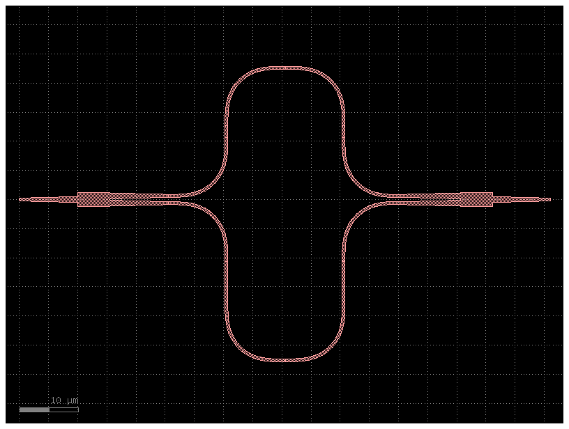
SAX gdsfactory Compatibility#
From Layout to Circuit Model
If you define your SAX S parameter models for your components, you can directly simulate your circuits from gdsfactory
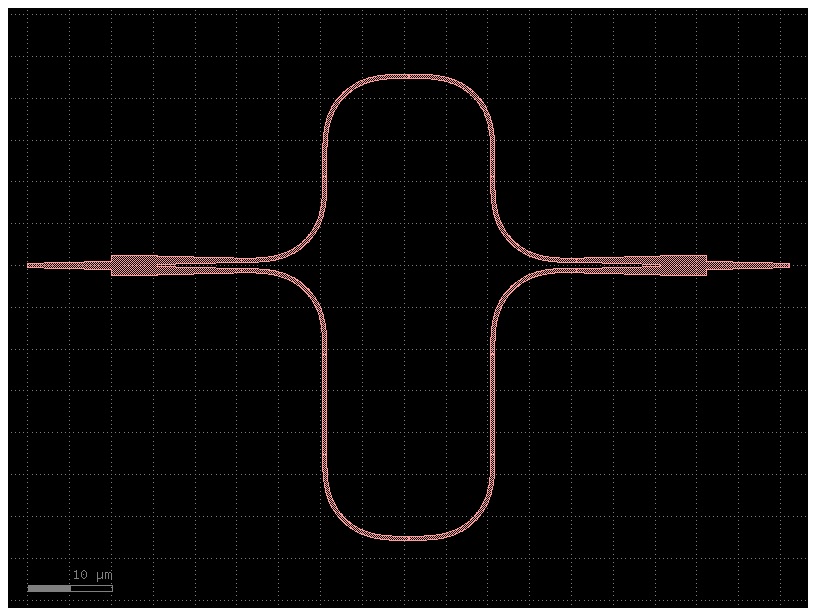
mzi = gf.components.mzi(delta_length=10)
mzi.plot()
netlist = mzi.get_netlist()
pprint(netlist["nets"])
({'p1': 'b1,o1', 'p2': 'cp1,o2'},
 {'p1': 'b1,o2', 'p2': 'sytl,o1'},
 {'p1': 'b2,o1', 'p2': 'sxt,o1'},
 {'p1': 'b2,o2', 'p2': 'sytl,o2'},
 {'p1': 'b3,o1', 'p2': 'sytr,o2'},
 {'p1': 'b3,o2', 'p2': 'sxt,o2'},
 {'p1': 'b4,o1', 'p2': 'sytr,o1'},
 {'p1': 'b4,o2', 'p2': 'cp2,o2'},
 {'p1': 'b5,o1', 'p2': 'cp1,o3'},
 {'p1': 'b5,o2', 'p2': 'syl,o1'},
 {'p1': 'b6,o1', 'p2': 'syl,o2'},
 {'p1': 'b6,o2', 'p2': 'sxb,o1'},
 {'p1': 'b7,o1', 'p2': 'sxb,o2'},
 {'p1': 'b7,o2', 'p2': 'sybr,o1'},
 {'p1': 'b8,o1', 'p2': 'cp2,o3'},
 {'p1': 'b8,o2', 'p2': 'sybr,o2'})
The netlist has three different components:
straight
mmi1x2
bend_euler
You need models for each subcomponents to simulate the Component.
def straight(wl=1.5, length=10.0, neff=2.4) -> sax.SDict:
    return sax.reciprocal({("o1", "o2"): jnp.exp(2j * jnp.pi * neff * length / wl)})


def mmi1x2():
    """Assumes a perfect 1x2 splitter"""
    return sax.reciprocal(
        {
            ("o1", "o2"): 0.5**0.5,
            ("o1", "o3"): 0.5**0.5,
        }
    )


def bend_euler(wl=1.5, length=20.0):
    """ "Let's assume a reduced transmission for the euler bend compared to a straight"""
    return {k: 0.99 * v for k, v in straight(wl=wl, length=length).items()}


models = {
    "bend_euler": bend_euler,
    "mmi1x2": mmi1x2,
    "straight": straight,
}
circuit, _ = sax.circuit(netlist=netlist, models=models)
circuit, _ = sax.circuit(netlist=netlist, models=models)
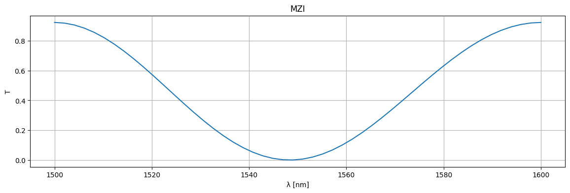
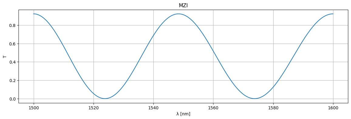
wl = np.linspace(1.5, 1.6)
S = circuit(wl=wl)
plt.figure(figsize=(14, 4))
plt.title("MZI")
plt.plot(1e3 * wl, jnp.abs(S["o1", "o2"]) ** 2)
plt.xlabel("λ [nm]")
plt.ylabel("T")
plt.grid(True)
plt.show()
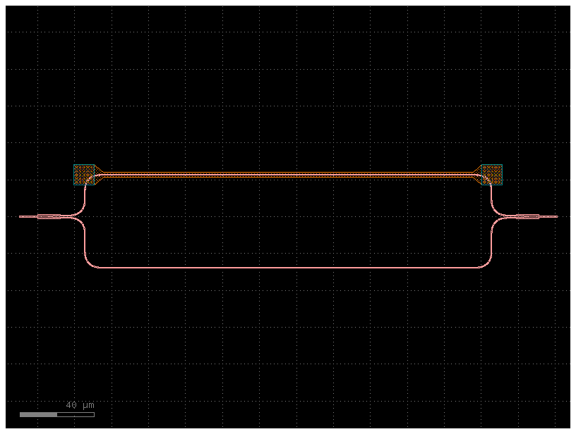
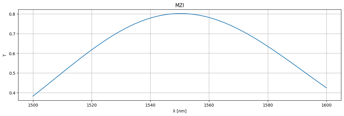
mzi = gf.components.mzi(delta_length=20)  # Double the length, reduces FSR by 1/2
mzi.plot()
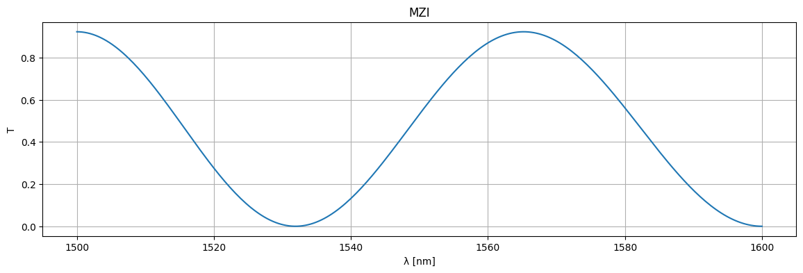
circuit, _ = sax.circuit(netlist=mzi.get_netlist(), models=models)

wl = np.linspace(1.5, 1.6, 256)
S = circuit(wl=wl)

plt.figure(figsize=(14, 4))
plt.title("MZI")
plt.plot(1e3 * wl, jnp.abs(S["o1", "o2"]) ** 2)
plt.xlabel("λ [nm]")
plt.ylabel("T")
plt.grid(True)
plt.show()
Heater model#
You can make a phase shifter model that depends on the applied volage. For that you need first to figure out what’s the model associated to your phase shifter, and what is the parameter that you need to tune.
delta_length = 10
mzi_component = gf.components.mzi_phase_shifter(delta_length=delta_length)
mzi_component.plot()
def straight(wl=1.5, length=10.0, neff=2.4) -> sax.SDict:
    return sax.reciprocal({("o1", "o2"): jnp.exp(2j * jnp.pi * neff * length / wl)})


def mmi1x2() -> sax.SDict:
    """Returns a perfect 1x2 splitter."""
    return sax.reciprocal(
        {
            ("o1", "o2"): 0.5**0.5,
            ("o1", "o3"): 0.5**0.5,
        }
    )


def bend_euler(wl=1.5, length=20.0) -> sax.SDict:
    """Returns bend Sparameters with reduced transmission compared to a straight."""
    return {k: 0.99 * v for k, v in straight(wl=wl, length=length).items()}


def phase_shifter_heater(
    wl: float = 1.55,
    neff: float = 2.34,
    voltage: float = 0,
    length: float = 10,
    loss: float = 0.0,
) -> sax.SDict:
    """Returns simple phase shifter model.

    Args:
        wl: wavelength.
        neff: effective index.
        voltage: voltage.
        length: length.
        loss: loss in dB/cm.
    """
    deltaphi = voltage * jnp.pi
    phase = 2 * jnp.pi * neff * length / wl + deltaphi
    amplitude = jnp.asarray(10 ** (-loss * length / 20), dtype=complex)
    transmission = amplitude * jnp.exp(1j * phase)
    return sax.reciprocal(
        {
            ("o1", "o2"): transmission,
            ("l_e1", "r_e1"): 0.0,
            ("l_e2", "r_e2"): 0.0,
            ("l_e3", "r_e3"): 0.0,
            ("l_e4", "r_e4"): 0.0,
        }
    )


models = {
    "bend_euler": bend_euler,
    "mmi1x2": mmi1x2,
    "straight": straight,
    "straight_heater_metal_undercut": phase_shifter_heater,
}
mzi_component = gf.components.mzi_phase_shifter(delta_length=delta_length)
netlist = mzi_component.get_netlist()
mzi_circuit, _ = sax.circuit(netlist=netlist, models=models)
S = mzi_circuit(wl=1.55)
S
{('e1', 'e1'): Array(0.+0.j, dtype=complex128),
 ('e1', 'e2'): Array(0.+0.j, dtype=complex128),
 ('e1', 'e3'): Array(0.+0.j, dtype=complex128),
 ('e1', 'e4'): Array(0.+0.j, dtype=complex128),
 ('e1', 'e5'): Array(0.+0.j, dtype=complex128),
 ('e1', 'e6'): Array(0.+0.j, dtype=complex128),
 ('e1', 'e7'): Array(0.+0.j, dtype=complex128),
 ('e1', 'e8'): Array(0.+0.j, dtype=complex128),
 ('e1', 'o1'): Array(0.+0.j, dtype=complex128),
 ('e1', 'o2'): Array(0.+0.j, dtype=complex128),
 ('e2', 'e1'): Array(0.+0.j, dtype=complex128),
 ('e2', 'e2'): Array(0.+0.j, dtype=complex128),
 ('e2', 'e3'): Array(0.+0.j, dtype=complex128),
 ('e2', 'e4'): Array(0.+0.j, dtype=complex128),
 ('e2', 'e5'): Array(0.+0.j, dtype=complex128),
 ('e2', 'e6'): Array(0.+0.j, dtype=complex128),
 ('e2', 'e7'): Array(0.+0.j, dtype=complex128),
 ('e2', 'e8'): Array(0.+0.j, dtype=complex128),
 ('e2', 'o1'): Array(0.+0.j, dtype=complex128),
 ('e2', 'o2'): Array(0.+0.j, dtype=complex128),
 ('e3', 'e1'): Array(0.+0.j, dtype=complex128),
 ('e3', 'e2'): Array(0.+0.j, dtype=complex128),
 ('e3', 'e3'): Array(0.+0.j, dtype=complex128),
 ('e3', 'e4'): Array(0.+0.j, dtype=complex128),
 ('e3', 'e5'): Array(0.+0.j, dtype=complex128),
 ('e3', 'e6'): Array(0.+0.j, dtype=complex128),
 ('e3', 'e7'): Array(0.+0.j, dtype=complex128),
 ('e3', 'e8'): Array(0.+0.j, dtype=complex128),
 ('e3', 'o1'): Array(0.+0.j, dtype=complex128),
 ('e3', 'o2'): Array(0.+0.j, dtype=complex128),
 ('e4', 'e1'): Array(0.+0.j, dtype=complex128),
 ('e4', 'e2'): Array(0.+0.j, dtype=complex128),
 ('e4', 'e3'): Array(0.+0.j, dtype=complex128),
 ('e4', 'e4'): Array(0.+0.j, dtype=complex128),
 ('e4', 'e5'): Array(0.+0.j, dtype=complex128),
 ('e4', 'e6'): Array(0.+0.j, dtype=complex128),
 ('e4', 'e7'): Array(0.+0.j, dtype=complex128),
 ('e4', 'e8'): Array(0.+0.j, dtype=complex128),
 ('e4', 'o1'): Array(0.+0.j, dtype=complex128),
 ('e4', 'o2'): Array(0.+0.j, dtype=complex128),
 ('e5', 'e1'): Array(0.+0.j, dtype=complex128),
 ('e5', 'e2'): Array(0.+0.j, dtype=complex128),
 ('e5', 'e3'): Array(0.+0.j, dtype=complex128),
 ('e5', 'e4'): Array(0.+0.j, dtype=complex128),
 ('e5', 'e5'): Array(0.+0.j, dtype=complex128),
 ('e5', 'e6'): Array(0.+0.j, dtype=complex128),
 ('e5', 'e7'): Array(0.+0.j, dtype=complex128),
 ('e5', 'e8'): Array(0.+0.j, dtype=complex128),
 ('e5', 'o1'): Array(0.+0.j, dtype=complex128),
 ('e5', 'o2'): Array(0.+0.j, dtype=complex128),
 ('e6', 'e1'): Array(0.+0.j, dtype=complex128),
 ('e6', 'e2'): Array(0.+0.j, dtype=complex128),
 ('e6', 'e3'): Array(0.+0.j, dtype=complex128),
 ('e6', 'e4'): Array(0.+0.j, dtype=complex128),
 ('e6', 'e5'): Array(0.+0.j, dtype=complex128),
 ('e6', 'e6'): Array(0.+0.j, dtype=complex128),
 ('e6', 'e7'): Array(0.+0.j, dtype=complex128),
 ('e6', 'e8'): Array(0.+0.j, dtype=complex128),
 ('e6', 'o1'): Array(0.+0.j, dtype=complex128),
 ('e6', 'o2'): Array(0.+0.j, dtype=complex128),
 ('e7', 'e1'): Array(0.+0.j, dtype=complex128),
 ('e7', 'e2'): Array(0.+0.j, dtype=complex128),
 ('e7', 'e3'): Array(0.+0.j, dtype=complex128),
 ('e7', 'e4'): Array(0.+0.j, dtype=complex128),
 ('e7', 'e5'): Array(0.+0.j, dtype=complex128),
 ('e7', 'e6'): Array(0.+0.j, dtype=complex128),
 ('e7', 'e7'): Array(0.+0.j, dtype=complex128),
 ('e7', 'e8'): Array(0.+0.j, dtype=complex128),
 ('e7', 'o1'): Array(0.+0.j, dtype=complex128),
 ('e7', 'o2'): Array(0.+0.j, dtype=complex128),
 ('e8', 'e1'): Array(0.+0.j, dtype=complex128),
 ('e8', 'e2'): Array(0.+0.j, dtype=complex128),
 ('e8', 'e3'): Array(0.+0.j, dtype=complex128),
 ('e8', 'e4'): Array(0.+0.j, dtype=complex128),
 ('e8', 'e5'): Array(0.+0.j, dtype=complex128),
 ('e8', 'e6'): Array(0.+0.j, dtype=complex128),
 ('e8', 'e7'): Array(0.+0.j, dtype=complex128),
 ('e8', 'e8'): Array(0.+0.j, dtype=complex128),
 ('e8', 'o1'): Array(0.+0.j, dtype=complex128),
 ('e8', 'o2'): Array(0.+0.j, dtype=complex128),
 ('o1', 'e1'): Array(0.+0.j, dtype=complex128),
 ('o1', 'e2'): Array(0.+0.j, dtype=complex128),
 ('o1', 'e3'): Array(0.+0.j, dtype=complex128),
 ('o1', 'e4'): Array(0.+0.j, dtype=complex128),
 ('o1', 'e5'): Array(0.+0.j, dtype=complex128),
 ('o1', 'e6'): Array(0.+0.j, dtype=complex128),
 ('o1', 'e7'): Array(0.+0.j, dtype=complex128),
 ('o1', 'e8'): Array(0.+0.j, dtype=complex128),
 ('o1', 'o1'): Array(0.+0.j, dtype=complex128),
 ('o1', 'o2'): Array(-0.15452351+0.71229167j, dtype=complex128),
 ('o2', 'e1'): Array(0.+0.j, dtype=complex128),
 ('o2', 'e2'): Array(0.+0.j, dtype=complex128),
 ('o2', 'e3'): Array(0.+0.j, dtype=complex128),
 ('o2', 'e4'): Array(0.+0.j, dtype=complex128),
 ('o2', 'e5'): Array(0.+0.j, dtype=complex128),
 ('o2', 'e6'): Array(0.+0.j, dtype=complex128),
 ('o2', 'e7'): Array(0.+0.j, dtype=complex128),
 ('o2', 'e8'): Array(0.+0.j, dtype=complex128),
 ('o2', 'o1'): Array(-0.15452351+0.71229167j, dtype=complex128),
 ('o2', 'o2'): Array(0.+0.j, dtype=complex128)}
wl = np.linspace(1.5, 1.6, 256)
S = mzi_circuit(wl=wl)

plt.figure(figsize=(14, 4))
plt.title("MZI")
plt.plot(1e3 * wl, jnp.abs(S["o1", "o2"]) ** 2)
plt.xlabel("λ [nm]")
plt.ylabel("T")
plt.grid(True)
plt.show()
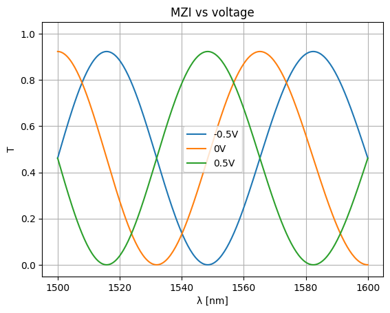
Now you can tune the phase shift applied to one of the arms.
How do you find out what’s the name of the netlist component that you want to tune?
You can backannotate the netlist and read the labels on the backannotated netlist or you can plot the netlist
mzi_component.plot_netlist()
<networkx.classes.graph.Graph at 0x7effcb8d9d60>
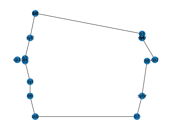
As you can see the top phase shifter instance sxt is hard to see on the netlist.
You can also reconstruct the component using the netlist and look at the labels in klayout.
mzi_yaml = mzi_component.get_netlist()
mzi_component2 = gf.read.from_yaml(mzi_yaml)
fig = mzi_component2.plot()
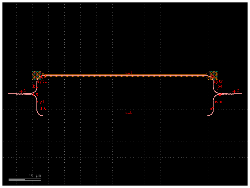
The best way to get a deterministic name of the instance is naming the reference on your Pcell.
voltages = np.linspace(-1, 1, num=5)
voltages = [-0.5, 0, 0.5]

for voltage in voltages:
    S = mzi_circuit(
        wl=wl,
        sxt={"voltage": voltage},
    )
    plt.plot(wl * 1e3, abs(S["o1", "o2"]) ** 2, label=f"{voltage}V")
    plt.xlabel("λ [nm]")
    plt.ylabel("T")
    plt.ylim(-0.05, 1.05)
    plt.grid(True)

plt.title("MZI vs voltage")
plt.legend()
<matplotlib.legend.Legend at 0x7effcb7aa8a0>
Variable splitter#
You can build a variable splitter by adding a delta length between two 50% power splitters

For example adding a 60um delta length you can build a 90% power splitter
@gf.cell
def variable_splitter(delta_length: float, splitter=gf.c.mmi2x2):
    return gf.c.mzi2x2_2x2(splitter=splitter, delta_length=delta_length)


nm = 1e-3
c = variable_splitter(delta_length=60 * nm)
c.plot()
models = {
    "bend_euler": gs.models.bend,
    "mmi2x2": gs.models.mmi2x2,
    "straight": gs.models.straight,
}

netlist = c.get_netlist()
circuit, _ = sax.circuit(netlist=netlist, models=models)
wl = np.linspace(1.5, 1.6)
S = circuit(wl=wl)

plt.figure(figsize=(14, 4))
plt.title("MZI")
plt.plot(1e3 * wl, jnp.abs(S["o1", "o3"]) ** 2, label="T")
plt.xlabel("λ [nm]")
plt.ylabel("T")
plt.grid(True)
plt.show()
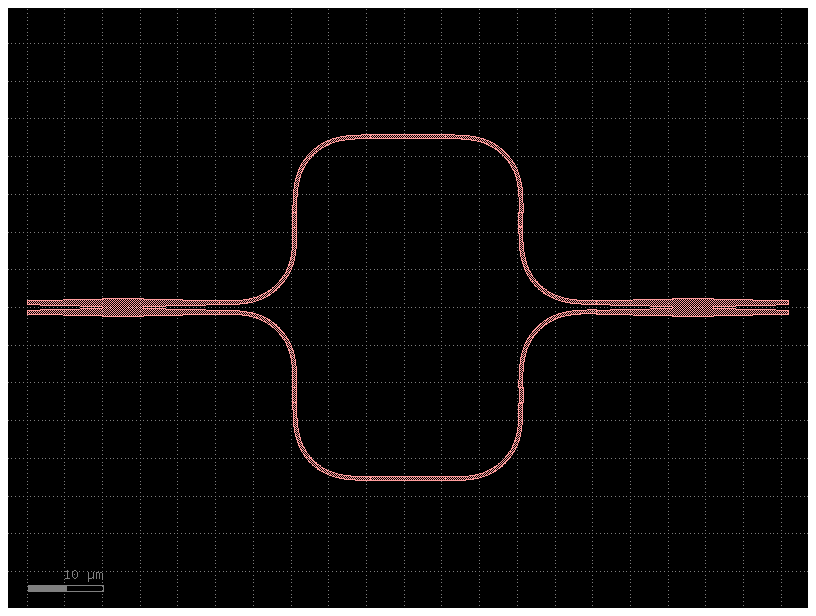
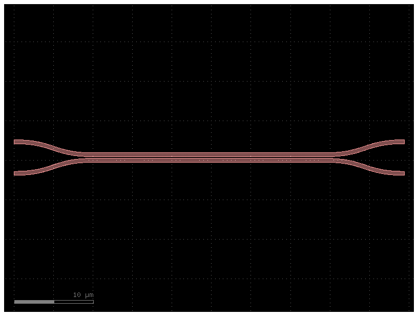
Coupler sim#
Lets compare one coupler versus two coupler
c = gf.components.coupler(length=29.4, gap=0.2)
c.plot()
coupler50 = partial(gs.models.coupler, dn=0.026, length=29.4 / 2, coupling0=0)
gs.plot_model(coupler50)
<Axes: title={'center': 'coupler S-Parameters'}, xlabel='wavelength (µm)', ylabel='|S (dB)|'>
As you can see the 50% coupling is only at one wavelength (1550nm)
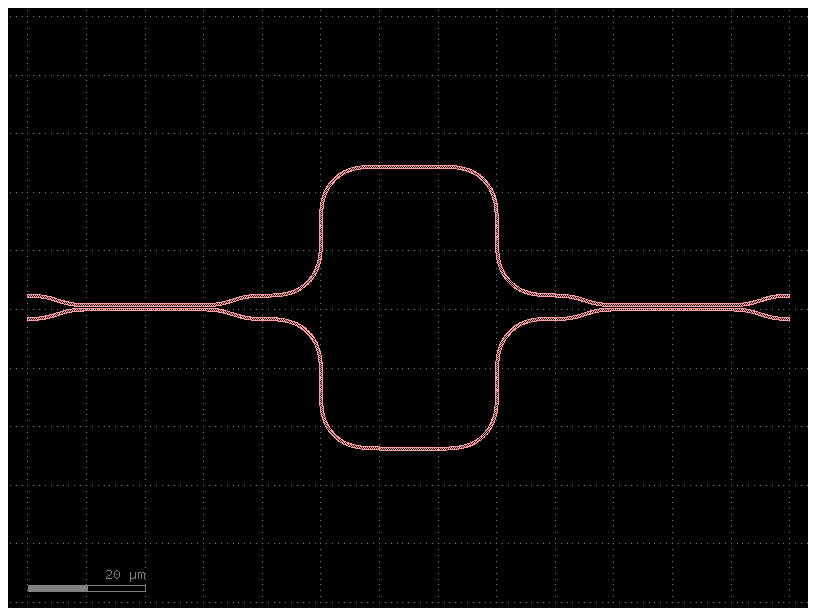
You can chain two couplers to increase the wavelength range for 50% operation.
@gf.cell
def broadband_coupler(delta_length=0, splitter=gf.c.coupler):
    return gf.c.mzi2x2_2x2(
        splitter=splitter, combiner=splitter, delta_length=delta_length
    )


c = broadband_coupler(delta_length=120 * nm)
c.plot()
c = broadband_coupler(delta_length=164 * nm)
models = {
    "bend_euler": gs.models.bend,
    "coupler": coupler50,
    "straight": gs.models.straight,
}

netlist = c.get_netlist()
circuit, _ = sax.circuit(netlist=netlist, models=models)
wl = np.linspace(1.5, 1.6)
S = circuit(wl=wl)

plt.figure(figsize=(14, 4))
plt.title("MZI")
# plt.plot(1e3 * wl, jnp.abs(S["o1", "o3"]) ** 2, label='T')
plt.plot(1e3 * wl, 20 * np.log10(jnp.abs(S["o1", "o3"])), label="T")
plt.plot(1e3 * wl, 20 * np.log10(jnp.abs(S["o1", "o4"])), label="K")
plt.xlabel("λ [nm]")
plt.ylabel("T")
plt.legend()
plt.grid(True)
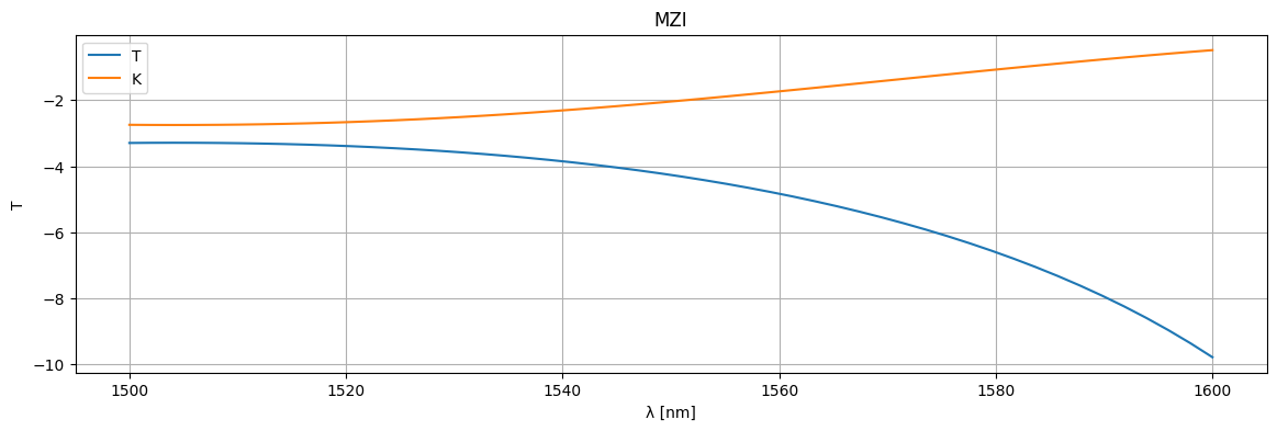
As you can see two couplers have more broadband response