Path and CrossSection

Path and CrossSection#

You can create a Path in gdsfactory and extrude it with an arbitrary CrossSection.

Lets create a path:

Create a blank Path.
Append points to the Path either using the built-in functions (arc(), straight(), euler() …) or by providing your own lists of points
Specify CrossSection with layers and offsets.
Extrude Path with a CrossSection to create a Component with the path polygons in it.

from functools import partial

import matplotlib.pyplot as plt
import numpy as np

import gdsfactory as gf
from gdsfactory.cross_section import Section

Path#

The first step is to generate the list of points we want the path to follow. Let’s start out by creating a blank Path and using the built-in functions to make a few smooth turns.

p1 = gf.path.straight(length=5)
p2 = gf.path.euler(radius=5, angle=45, p=0.5, use_eff=False)
p = p1 + p2
f = p.plot()

Ignoring fixed y limits to fulfill fixed data aspect with adjustable data limits.

../_images/e578b874ca3c0305bec1bd39d40bf13ae4fd538d4c387cb82b4aa36667d73a10.png

p1 = gf.path.straight(length=5)
p2 = gf.path.euler(radius=5, angle=45, p=0.5, use_eff=False)
p = p2 + p1
f = p.plot()

Ignoring fixed y limits to fulfill fixed data aspect with adjustable data limits.

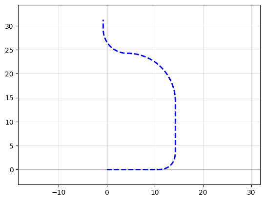
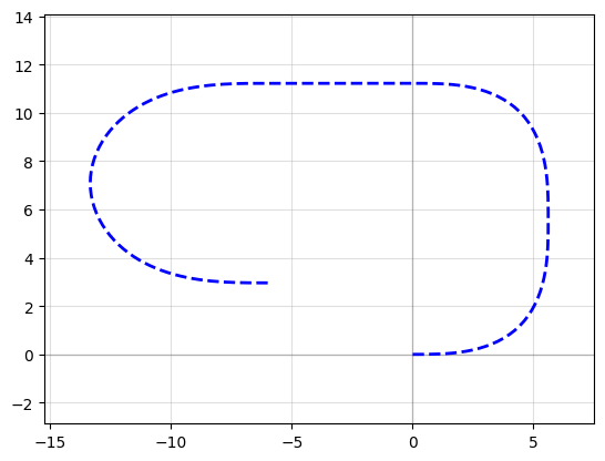
../_images/89ed46a90f4e093d4cdd722cb977c91d1b14dc5643f4cdb6e1fb93a3c7257722.png

P = gf.Path()
P += gf.path.arc(radius=10, angle=90)  # Circular arc
P += gf.path.straight(length=10)  # Straight section
P += gf.path.euler(radius=3, angle=-90)  # Euler bend (aka "racetrack" curve)
P += gf.path.straight(length=40)
P += gf.path.arc(radius=8, angle=-45)
P += gf.path.straight(length=10)
P += gf.path.arc(radius=8, angle=45)
P += gf.path.straight(length=10)

f = P.plot()

Ignoring fixed y limits to fulfill fixed data aspect with adjustable data limits.

../_images/3d7a9a61ab6c1fee6af52106451ad4dd9684146a4c2e7c01583c615b9bfa865d.png

p2 = P.copy().rotate()
f = p2.plot()

Ignoring fixed x limits to fulfill fixed data aspect with adjustable data limits.

../_images/86b1568b5ab8854c4dde7e5efff8dc6482f713b3444d137d15793f693538ef79.png

P.points - p2.points

array([[  0.        ,   0.        ],
       [  0.07775818,  -0.18109421],
       [  0.16015338,  -0.36012627],
       [  0.24713097,  -0.53697746],
       [  0.33863327,  -0.71153054],
       [  0.43459961,  -0.88366975],
       [  0.53496636,  -1.05328096],
       [  0.63966697,  -1.2202517 ],
       [  0.74863202,  -1.38447127],
       [  0.86178925,  -1.54583076],
       [  0.97906364,  -1.7042232 ],
       [  1.10037742,  -1.85954356],
       [  1.22565016,  -2.01168884],
       [  1.35479879,  -2.16055818],
       [  1.48773767,  -2.30605285],
       [  1.62437867,  -2.44807638],
       [  1.76463118,  -2.58653461],
       [  1.9084022 ,  -2.72133573],
       [  2.0555964 ,  -2.85239035],
       [  2.20611618,  -2.97961158],
       [  2.35986175,  -3.10291506],
       [  2.51673115,  -3.22221903],
       [  2.67662037,  -3.33744439],
       [  2.83942339,  -3.44851474],
       [  3.00503227,  -3.55535642],
       [  3.1733372 ,  -3.6578986 ],
       [  3.34422657,  -3.75607328],
       [  3.51758709,  -3.84981537],
       [  3.69330379,  -3.93906271],
       [  3.87126017,  -4.02375613],
       [  4.05133823,  -4.10383946],
       [  4.23341856,  -4.1792596 ],
       [  4.41738044,  -4.24996655],
       [  4.60310189,  -4.31591343],
       [  4.79045976,  -4.3770565 ],
       [  4.97932982,  -4.43335522],
       [  5.16958684,  -4.48477228],
       [  5.36110467,  -4.53127356],
       [  5.55375631,  -4.57282824],
       [  5.74741403,  -4.60940877],
       [  5.94194941,  -4.64099089],
       [  6.13723348,  -4.66755366],
       [  6.33313674,  -4.68907946],
       [  6.52952929,  -4.70555403],
       [  6.72628092,  -4.71696644],
       [  6.92326117,  -4.72330911],
       [  7.12033942,  -4.72457786],
       [  7.317385  ,  -4.72077183],
       [  7.51426725,  -4.71189355],
       [  7.71085564,  -4.69794891],
       [  7.90701981,  -4.67894715],
       [  8.10262968,  -4.65490087],
       [  8.29755556,  -4.62582602],
       [  8.4916682 ,  -4.59174187],
       [  8.6848389 ,  -4.55267103],
       [  8.87693955,  -4.50863939],
       [  9.0678428 ,  -4.45967617],
       [  9.25742205,  -4.40581381],
       [  9.44555161,  -4.34708805],
       [  9.63210673,  -4.28353781],
       [  9.81696372,  -4.21520523],
       [ 10.        ,  -4.14213562],
       [ 17.07106781,  -1.21320344],
       [ 17.22259744,  -1.15062977],
       [ 17.3745295 ,  -1.0890412 ],
       [ 17.52724719,  -1.02943054],
       [ 17.68109502,  -0.9728054 ],
       [ 17.83635884,  -0.92019408],
       [ 17.99324531,  -0.87264941],
       [ 18.15186066,  -0.83125013],
       [ 18.31218874,  -0.79709882],
       [ 18.47406876,  -0.77131591],
       [ 18.63717281,  -0.75502883],
       [ 18.80098407,  -0.74935572],
       [ 18.98113405,  -0.75643383],
       [ 19.16017334,  -0.77762453],
       [ 19.33699811,  -0.81279716],
       [ 19.51051817,  -0.86173488],
       [ 19.67966373,  -0.92413597],
       [ 19.84339193,  -0.9996157 ],
       [ 20.00069333,  -1.08770872],
       [ 20.15059814,  -1.18787191],
       [ 20.29218212,  -1.29948772],
       [ 20.42457237,  -1.42186801],
       [ 20.53639293,  -1.54171156],
       [ 20.6402082 ,  -1.66856024],
       [ 20.73644339,  -1.80125797],
       [ 20.82566384,  -1.93877567],
       [ 20.90854811,  -2.08020737],
       [ 20.98586445,  -2.22476202],
       [ 21.05845073,  -2.37175194],
       [ 21.12719755,  -2.5205788 ],
       [ 21.19303416,  -2.67071762],
       [ 21.25691665,  -2.82169951],
       [ 21.31981802,  -2.97309339],
       [ 33.03554677, -31.25736464],
       [ 33.1091836 , -31.44370627],
       [ 33.17668408, -31.63235747],
       [ 33.23797592, -31.82311621],
       [ 33.29299349, -32.01577822],
       [ 33.34167789, -32.21013721],
       [ 33.38397696, -32.40598505],
       [ 33.41984543, -32.60311201],
       [ 33.44924488, -32.80130701],
       [ 33.47214384, -33.00035782],
       [ 33.48851777, -33.20005129],
       [ 33.49834914, -33.40017358],
       [ 33.50162744, -33.60051039],
       [ 33.49834914, -33.80084721],
       [ 33.48851777, -34.0009695 ],
       [ 33.47214384, -34.20066296],
       [ 33.44924488, -34.39971377],
       [ 33.41984543, -34.59790877],
       [ 33.38397696, -34.79503574],
       [ 33.34167789, -34.99088357],
       [ 33.29299349, -35.18524256],
       [ 33.23797592, -35.37790458],
       [ 33.17668408, -35.56866332],
       [ 33.1091836 , -35.75731451],
       [ 33.03554677, -35.94365614],
       [ 30.10661458, -43.01472396],
       [ 30.03297776, -43.20106559],
       [ 29.96547728, -43.38971678],
       [ 29.90418544, -43.58047552],
       [ 29.84916786, -43.77313754],
       [ 29.80048347, -43.96749653],
       [ 29.75818439, -44.16334436],
       [ 29.72231592, -44.36047132],
       [ 29.69291647, -44.55866633],
       [ 29.67001752, -44.75771713],
       [ 29.65364359, -44.9574106 ],
       [ 29.64381221, -45.15753289],
       [ 29.64053392, -45.35786971],
       [ 29.64381221, -45.55820652],
       [ 29.65364359, -45.75832881],
       [ 29.67001752, -45.95802228],
       [ 29.69291647, -46.15707309],
       [ 29.72231592, -46.35526809],
       [ 29.75818439, -46.55239505],
       [ 29.80048347, -46.74824289],
       [ 29.84916786, -46.94260187],
       [ 29.90418544, -47.13526389],
       [ 29.96547728, -47.32602263],
       [ 30.03297776, -47.51467382],
       [ 30.10661458, -47.70101546],
       [ 33.03554677, -54.77208327]])

You can also modify our Path in the same ways as any other gdsfactory object:

Manipulation with move(), rotate(), mirror(), etc
Accessing properties like xmin, y, center, bbox, etc

P.movey(10)
P.xmin = 20
f = P.plot()

Ignoring fixed y limits to fulfill fixed data aspect with adjustable data limits.

../_images/5d00797e727a8c1ece1a9d3ebaff508a6873bfbeac71383dab3b1cb5afbcb6c0.png

You can also check the length of the curve with the length() method:

P.length()

105.34098399267245

CrossSection#

Now that you’ve got your path defined, the next step is to define the cross-section of the path. To do this, you can create a blank CrossSection and add whatever cross-sections you want to it. You can then combine the Path and the CrossSection using the gf.path.extrude() function to generate a Component:

Option 1: Single layer and width cross-section#

The simplest option is to just set the cross-section to be a constant width by passing a number to extrude() like so:

# Extrude the Path and the CrossSection
c = gf.path.extrude(P, layer=(1, 0), width=1.5)
c.plot()

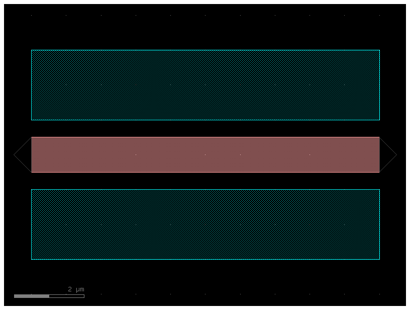
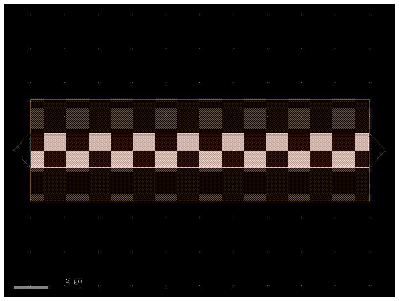
../_images/b6048025f9485fa86d415e53355e063939d69ba1c1b9986f4f03e4abd395e34c.png

Option 2: Arbitrary Cross-section#

You can also extrude an arbitrary cross_section

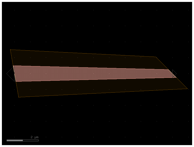
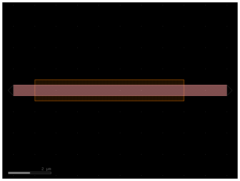
Now, what if we want a more complicated straight? For instance, in some photonic applications it’s helpful to have a shallow etch that appears on either side of the straight (often called a trench or sleeve). Additionally, it might be nice to have a Port on either end of the center section so we can snap other geometries to it. Let’s try adding something like that in:

p = gf.path.straight()

# Add a few "sections" to the cross-section
s0 = gf.Section(width=1, offset=0, layer=(1, 0), port_names=("in", "out"))
s1 = gf.Section(width=2, offset=2, layer=(2, 0))
s2 = gf.Section(width=2, offset=-2, layer=(2, 0))
x = gf.CrossSection(sections=[s0, s1, s2])

c = gf.path.extrude(p, cross_section=x)
c.plot()

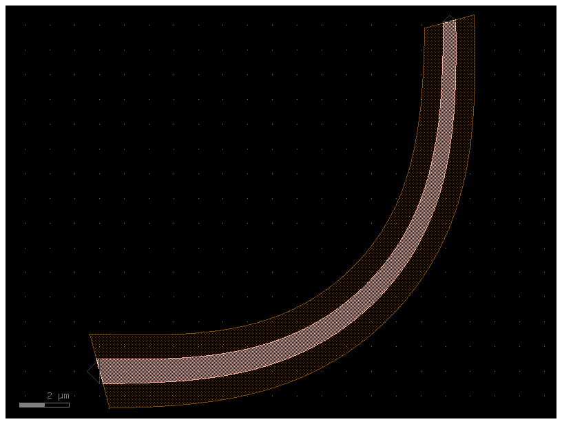
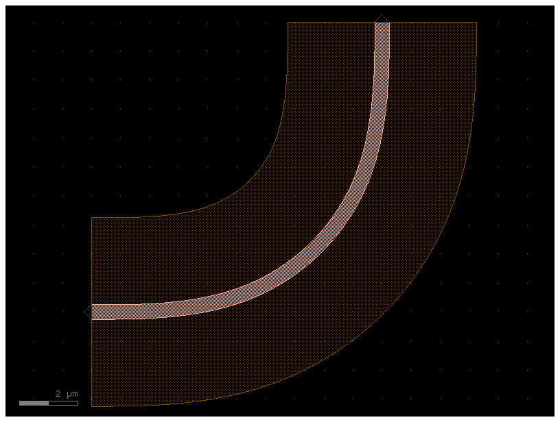
../_images/1016b8c0aad2aab8e629fb869699fcc263bc8544cfedfd51cca33a9a68ec0b7b.png

p = gf.path.arc()

# Combine the Path and the CrossSection
b = gf.path.extrude(p, cross_section=x)
b.plot()

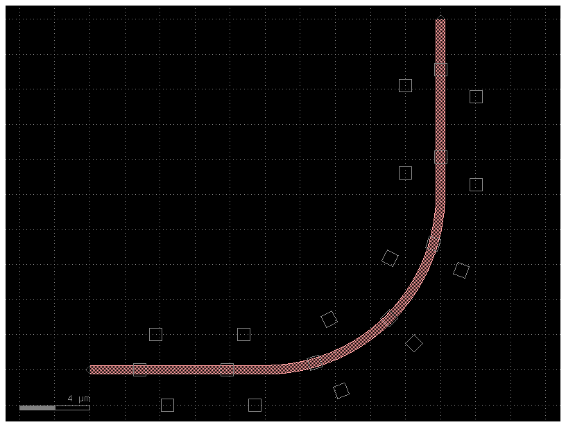
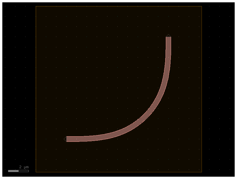
../_images/6fa35fa5a58009939996029b0a57bc7e14373d3731570115a86d9133a5392678.png

Option 3: CrossSection with ComponentAlongPath#

You can also place components along a path, which is useful for wiring vias.

import gdsfactory as gf
from gdsfactory.cross_section import ComponentAlongPath

# Create the path
p = gf.path.straight()
p += gf.path.arc(10)
p += gf.path.straight()

# Define a cross-section with a via
via = ComponentAlongPath(
    component=gf.c.rectangle(size=(1, 1), centered=True), spacing=5, padding=2
)
s = gf.Section(width=0.5, offset=0, layer=(1, 0), port_names=("in", "out"))
x = gf.CrossSection(sections=[s], components_along_path=[via])

# Combine the path with the cross-section
c = gf.path.extrude(p, cross_section=x)
c.plot()

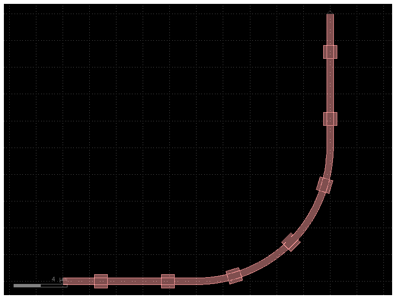
../_images/680d207028c9dec06ea45fbff4d36419f9a8a6367e5bab2e40d8d9a54d935a3e.png

import gdsfactory as gf
from gdsfactory.cross_section import ComponentAlongPath

# Create the path
p = gf.path.straight()
p += gf.path.arc(10)
p += gf.path.straight()

# Define a cross-section with a via
via0 = ComponentAlongPath(component=gf.c.via1(), spacing=5, padding=2, offset=0)
viap = ComponentAlongPath(component=gf.c.via1(), spacing=5, padding=2, offset=+2)
vian = ComponentAlongPath(component=gf.c.via1(), spacing=5, padding=2, offset=-2)
x = gf.CrossSection(sections=[s], components_along_path=[via0, viap, vian])

# Combine the path with the cross-section
c = gf.path.extrude(p, cross_section=x)
c.plot()

../_images/12182b65560457148280dc7e6b6cfacaca56014a798e206a17e940dec26d0862.png

Path#

You can pass append() lists of path segments. This makes it easy to combine paths very quickly. Below we show 3 examples using this functionality:

Example 1: Assemble a complex path by making a list of Paths and passing it to append()

P = gf.Path()

# Create the basic Path components
left_turn = gf.path.euler(radius=4, angle=90)
right_turn = gf.path.euler(radius=4, angle=-90)
straight = gf.path.straight(length=10)

# Assemble a complex path by making list of Paths and passing it to `append()`
P.append(
    [
        straight,
        left_turn,
        straight,
        right_turn,
        straight,
        straight,
        right_turn,
        left_turn,
        straight,
    ]
)

f = P.plot()

Ignoring fixed y limits to fulfill fixed data aspect with adjustable data limits.

../_images/cfffd66468e5f94bd638f65bbbe74bb9bebb73d2e8f4142a86af5b00321c2c92.png

P = (
    straight
    + left_turn
    + straight
    + right_turn
    + straight
    + straight
    + right_turn
    + left_turn
    + straight
)
f = P.plot()

Ignoring fixed y limits to fulfill fixed data aspect with adjustable data limits.

../_images/bbb2d7b551d0ee63aea83caeee01ac62d995c384bcb318bcf08bb7ecd1b3cf4b.png

Example 2: Create an “S-turn” just by making a list of [left_turn, right_turn]

P = gf.Path()

# Create an "S-turn" just by making a list
s_turn = [left_turn, right_turn]

P.append(s_turn)
f = P.plot()

Ignoring fixed x limits to fulfill fixed data aspect with adjustable data limits.

../_images/f4ca4a5240a7ce064463f51ab0c7d9c7a31d52efaf8e3c3421bb596feda05a14.png

Example 3: Repeat the S-turn 3 times by nesting our S-turn list in another list

P = gf.Path()

# Create an "S-turn" using a list
s_turn = [left_turn, right_turn]

# Repeat the S-turn 3 times by nesting our S-turn list 3x times in another list
triple_s_turn = [s_turn, s_turn, s_turn]

P.append(triple_s_turn)
f = P.plot()

Ignoring fixed x limits to fulfill fixed data aspect with adjustable data limits.

../_images/ff6367d5cbcbd67cd09786ab21526d4908b510a68fbae8179abf2c77c81d0cae.png

Note you can also use the Path() constructor to immediately construct your Path:

P = gf.Path([straight, left_turn, straight, right_turn, straight])
f = P.plot()

Ignoring fixed x limits to fulfill fixed data aspect with adjustable data limits.

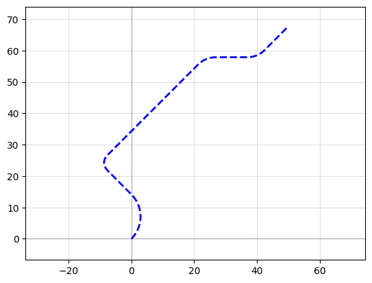
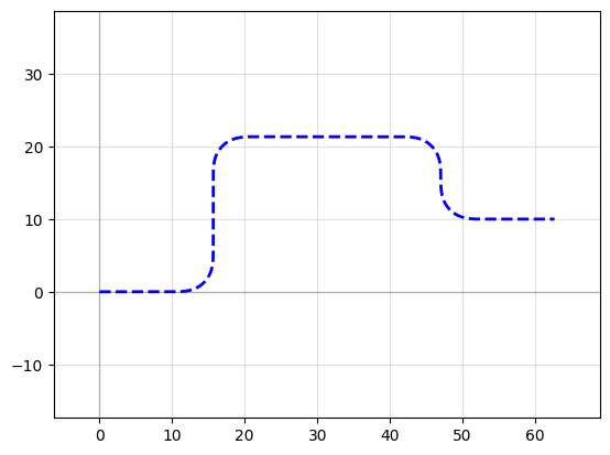
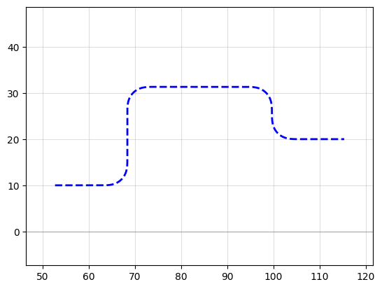
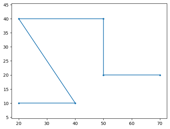
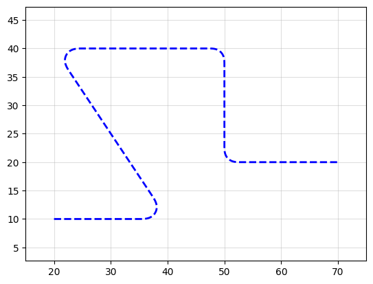
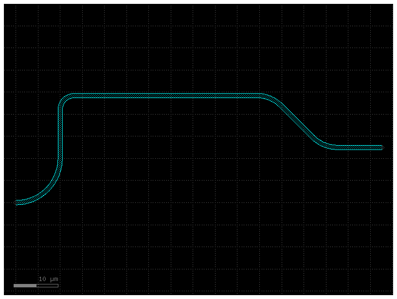
../_images/65962f47698bcdad2c271c8acc28df6669e1126d8d1895b4fdd5161d26a3d8a5.png

Waypoint smooth paths#

You can also build smooth paths between waypoints with the smooth() function

points = np.array([(20, 10), (40, 10), (20, 40), (50, 40), (50, 20), (70, 20)])
plt.plot(points[:, 0], points[:, 1], ".-")
plt.axis("equal")

(17.5, 72.5, 8.5, 41.5)

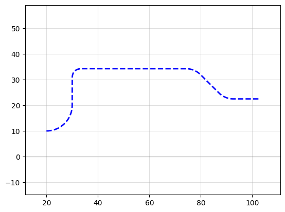
../_images/21323afb8f2c7c15e72483a03c0d9f1901b3c8316295cf84c6500f77456752cc.png

points = np.array([(20, 10), (40, 10), (20, 40), (50, 40), (50, 20), (70, 20)])

P = gf.path.smooth(
    points=points,
    radius=2,
    bend=gf.path.euler,  # Alternatively, use pp.arc
    use_eff=False,
)
f = P.plot()

Ignoring fixed y limits to fulfill fixed data aspect with adjustable data limits.

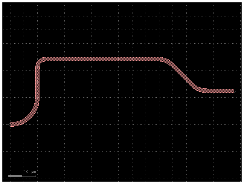
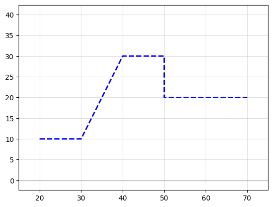
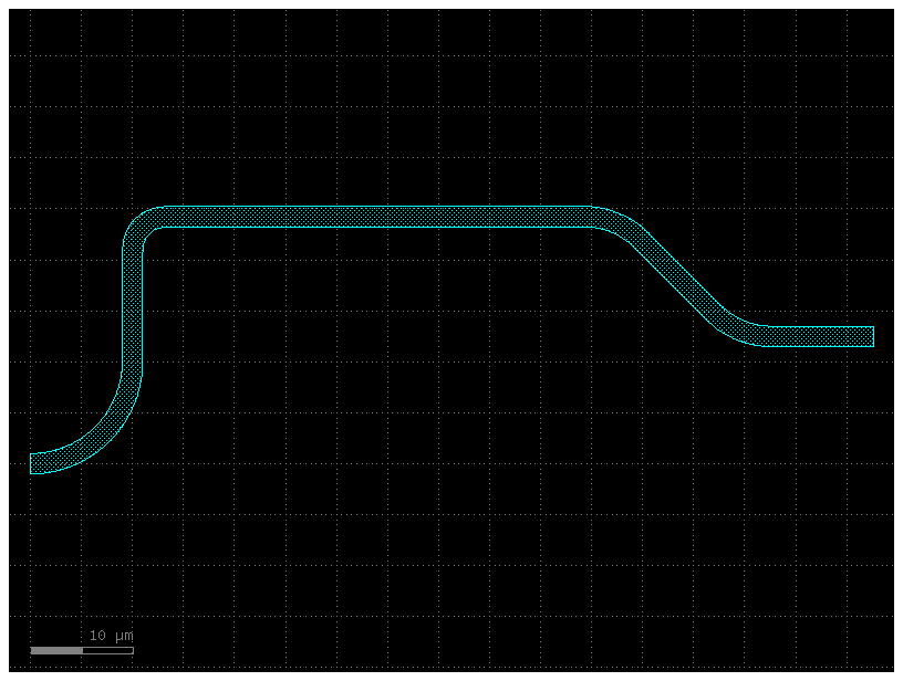
../_images/0f4de0131d3601786bfaa45a06ab905cd27a46016a180499d599b85460239db5.png

Waypoint sharp paths#

It’s also possible to make more traditional angular paths (e.g. electrical wires) in a few different ways.

Example 1: Using a simple list of points

P = gf.Path([(20, 10), (30, 10), (40, 30), (50, 30), (50, 20), (70, 20)])
f = P.plot()

Ignoring fixed y limits to fulfill fixed data aspect with adjustable data limits.

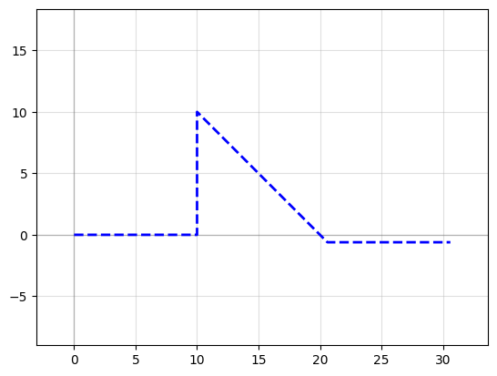
../_images/f9fd384926d098d011352defc07e0e6fbc8abd84bc0771360b62e35b446c3e97.png

Example 2: Using the “turn and move” method, where you manipulate the end angle of the Path so that when you append points to it, they’re in the correct direction. Note: It is crucial that the number of points per straight section is set to 2 (gf.path.straight(length, num_pts = 2)) otherwise the extrusion algorithm will show defects.

P = gf.Path()
P += gf.path.straight(length=10, npoints=2)
P.end_angle += 90  # "Turn" 90 deg (left)
P += gf.path.straight(length=10, npoints=2)  # "Walk" length of 10
P.end_angle += -135  # "Turn" -135 degrees (right)
P += gf.path.straight(length=15, npoints=2)  # "Walk" length of 10
P.end_angle = 0  # Force the direction to be 0 degrees
P += gf.path.straight(length=10, npoints=2)  # "Walk" length of 10
f = P.plot()

Ignoring fixed y limits to fulfill fixed data aspect with adjustable data limits.

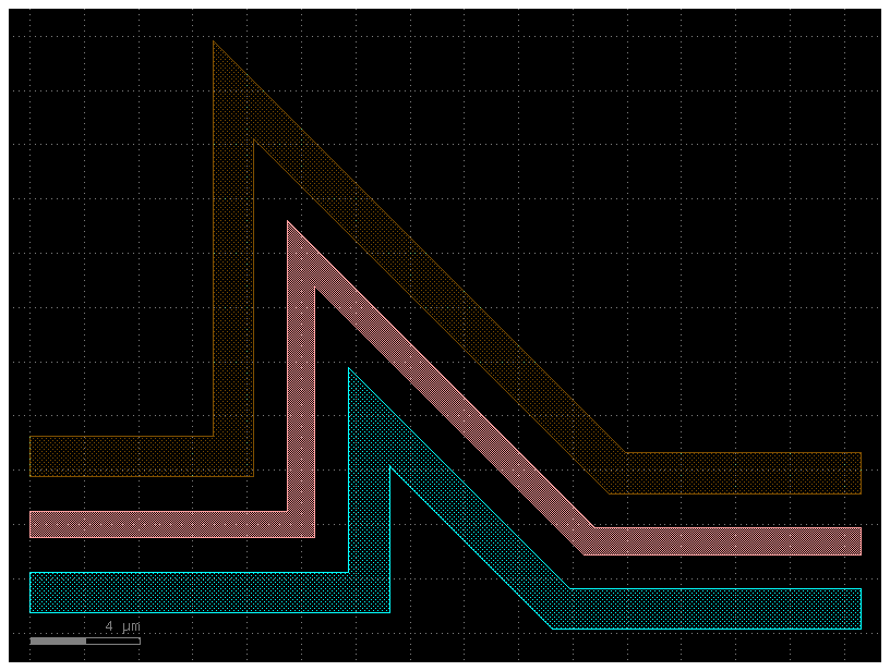
../_images/13df1b3fc38194b163228996bb12469b23da82e6d70c88f0c1e71c362c619071.png

s0 = gf.Section(width=1, offset=0, layer=(1, 0))
s1 = gf.Section(width=1.5, offset=2.5, layer=(2, 0))
s2 = gf.Section(width=1.5, offset=-2.5, layer=(3, 0))
X = gf.CrossSection(sections=[s0, s1, s2])
c = gf.path.extrude(P, X)
c.show()
c.plot()

2025-01-19 23:48:29.951 | WARNING  | gdsfactory.klive:show:49 - UserWarning: Could not connect to klive server. Is klayout open and klive plugin installed?

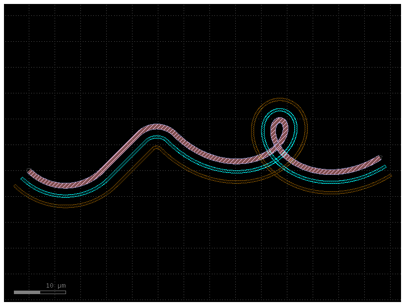
../_images/c1f8d234be9f92e44c03b8a23d82c9e2c800ef68f92c9840cccca57990fcd5c1.png

Custom curves#

Now let’s have some fun and try to make a loop-de-loop structure with parallel straights and several Ports.

To create a new type of curve we simply make a function that produces an array of points. The best way to do that is to create a function which allows you to specify a large number of points along that curve – in the case below, the looploop() function outputs 1000 points along a looping path. Later, if we want reduce the number of points in our geometry we can trivially simplify the path.

def looploop(num_pts=1000):
    """Simple limacon looping curve"""
    t = np.linspace(-np.pi, 0, num_pts)
    r = 20 + 25 * np.sin(t)
    x = r * np.cos(t)
    y = r * np.sin(t)
    return np.array((x, y)).T


# Create the path points
P = gf.Path()
P.append(gf.path.arc(radius=10, angle=90))
P.append(gf.path.straight())
P.append(gf.path.arc(radius=5, angle=-90))
P.append(looploop(num_pts=1000))
P.rotate(-45)

# Create the crosssection
s0 = gf.Section(width=1, offset=0, layer=(1, 0), port_names=("in", "out"))
s1 = gf.Section(width=0.5, offset=2, layer=(2, 0))
s2 = gf.Section(width=0.5, offset=4, layer=(3, 0))
s3 = gf.Section(width=1, offset=0, layer=(4, 0))
X = gf.CrossSection(sections=[s0, s1, s2, s3])

c = gf.path.extrude(P, X)
c.plot()

../_images/94cc9cc615c02592259c53d8aa11fad9d5f02980fd3e2c3c7d8a74f56b72cbcf.png

You can create Paths from any array of points – just be sure that they form smooth curves! If we examine our path P we can see that all we’ve simply created a long list of points:

path_points = P.points  # Curve points are stored as a numpy array in P.points
print(np.shape(path_points))  # The shape of the array is Nx2
print(len(P))  # Equivalently, use len(P) to see how many points are inside

(1092, 2)
1092

Simplifying / reducing point usage#

One of the chief concerns of generating smooth curves is that too many points are generated, inflating file sizes and making boolean operations computationally expensive. Fortunately, PHIDL has a fast implementation of the Ramer-Douglas–Peucker algorithm that lets you reduce the number of points in a curve without changing its shape. All that needs to be done is when you made a component component() extruding the path with a cross_section, you specify the simplify argument.

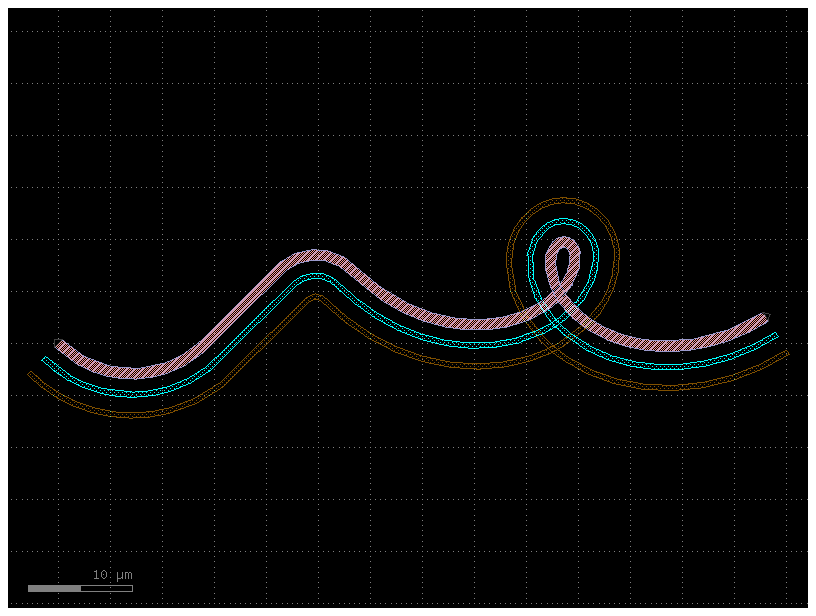
If we specify simplify = 1e-3, the number of points in the line drops from 12,000 to 4,000, and the remaining points form a line that is identical to within 1e-3 distance from the original (for the default 1 micron unit size, this corresponds to 1 nanometer resolution):

# The remaining points form a identical line to within `1e-3` from the original
c = gf.path.extrude(p=P, cross_section=X, simplify=1e-3)
c.plot()

../_images/30a28129716f7b7d66fdbed39df80399f9b71ae8000bbc2d0b7992b8120d1c07.png

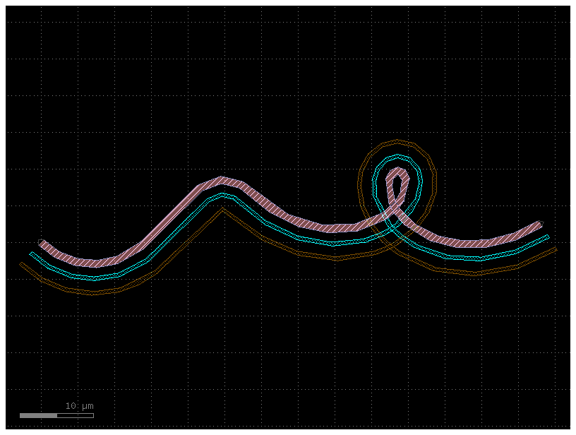
Let’s say we need fewer points. We can increase the simplify tolerance by specifying simplify = 1e-1. This drops the number of points to ~400 points form a line that is identical to within 1e-1 distance from the original:

c = gf.path.extrude(P, cross_section=X, simplify=1e-1)
c.plot()

../_images/8cd9ed9cd7fabc9eceb49d754cea09d914d86b1c5c5e93740f69f24d66fda565.png

Taken to absurdity, what happens if we set simplify = 0.3? Once again, the ~200 remaining points form a line that is within 0.3 units from the original – but that line looks pretty bad.

c = gf.path.extrude(P, cross_section=X, simplify=0.3)
c.plot()

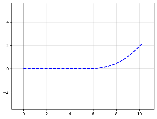
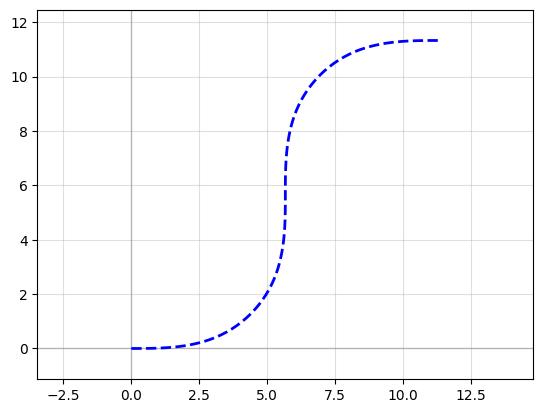
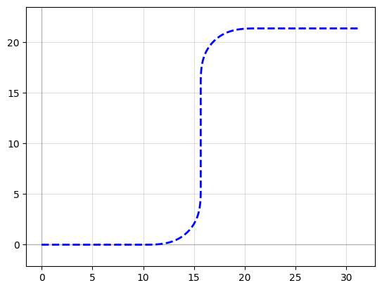
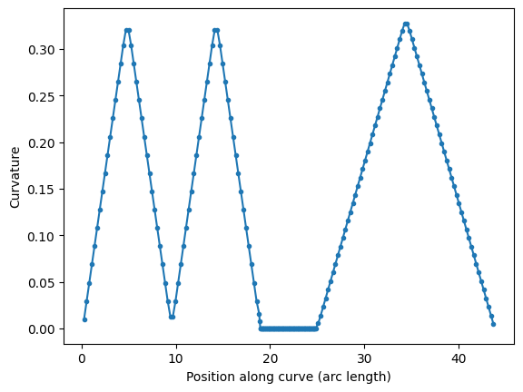
../_images/1eb05aa83b156f623b4873f2a630071d808a3a35df974ae948955742944bb65d.png

Curvature calculation#

The Path class has a curvature() method that computes the curvature K of your smooth path (K = 1/(radius of curvature)). This can be helpful for verifying that your curves transition smoothly such as in track-transition curves (also known as “Euler” bends in the photonics world). Euler bends have lower mode-mismatch loss as explained in this paper

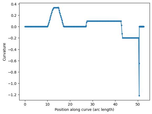
Note this curvature is numerically computed so areas where the curvature jumps instantaneously (such as between an arc and a straight segment) will be slightly interpolated, and sudden changes in point density along the curve can cause discontinuities.

straight_points = 100

P = gf.Path()
P.append(
    [
        gf.path.straight(
            length=10, npoints=straight_points
        ),  # Should have a curvature of 0
        gf.path.euler(
            radius=3, angle=90, p=0.5, use_eff=False
        ),  # Euler straight-to-bend transition with min. bend radius of 3 (max curvature of 1/3)
        gf.path.straight(
            length=10, npoints=straight_points
        ),  # Should have a curvature of 0
        gf.path.arc(radius=10, angle=90),  # Should have a curvature of 1/10
        gf.path.arc(radius=5, angle=-90),  # Should have a curvature of -1/5
        gf.path.straight(
            length=2, npoints=straight_points
        ),  # Should have a curvature of 0
    ]
)

f = P.plot()

Ignoring fixed x limits to fulfill fixed data aspect with adjustable data limits.

../_images/2693318712ddacba31ddf3f7bbb388686d2a745e06d05b3dee2c37d2813cf4a6.png

Arc paths are equivalent to bend_circular and euler paths are equivalent to bend_euler

s, K = P.curvature()
plt.plot(s, K, ".-")
plt.xlabel("Position along curve (arc length)")
plt.ylabel("Curvature")

Text(0, 0.5, 'Curvature')

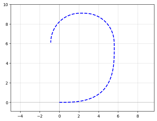
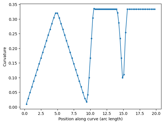
../_images/c4666a279d02de3eab277c0de2a6fda9f4b8f0066cd9487d5abcc53121197916.png

P = gf.path.euler(radius=3, angle=90, p=1.0, use_eff=False)
P.append(gf.path.euler(radius=3, angle=90, p=0.2, use_eff=False))
P.append(gf.path.euler(radius=3, angle=90, p=0.0, use_eff=False))
P.plot()

Ignoring fixed x limits to fulfill fixed data aspect with adjustable data limits.

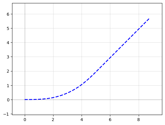
../_images/41dae17a5188dd04208f0b48a9ca4b9927927b9572583b5e03382c04241580eb.png

s, K = P.curvature()
plt.plot(s, K, ".-")
plt.xlabel("Position along curve (arc length)")
plt.ylabel("Curvature")

Text(0, 0.5, 'Curvature')

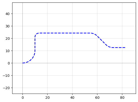
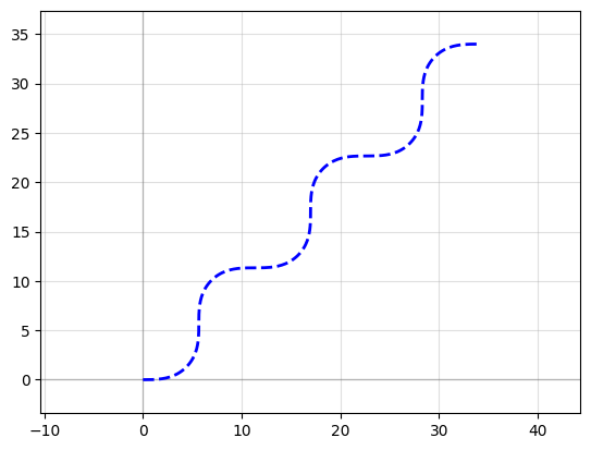
../_images/2f31ce144a2d388da79030c24da1ee2317ef5ef212f17e1a8b47366d477f200f.png

You can compare two 90 degrees euler bend with 180 euler bend.

A 180 euler bend is shorter, and has less loss than two 90 degrees euler bend.

straight_points = 100

P = gf.Path()
P.append(
    [
        gf.path.euler(radius=3, angle=90, p=1, use_eff=False),
        gf.path.euler(radius=3, angle=90, p=1, use_eff=False),
        gf.path.straight(length=6, npoints=100),
        gf.path.euler(radius=3, angle=180, p=1, use_eff=False),
    ]
)

f = P.plot()

Ignoring fixed y limits to fulfill fixed data aspect with adjustable data limits.

../_images/74b0fd142823989cad103efc7231b78797d59343d1ffe48fe12a16b87a059aaf.png

s, K = P.curvature()
plt.plot(s, K, ".-")
plt.xlabel("Position along curve (arc length)")
plt.ylabel("Curvature")

Text(0, 0.5, 'Curvature')

../_images/6d14708866ddf79361517cc3e28561b0c3d16279e7e4a2e55ccd01b229c7a79a.png

Transitioning between cross-sections#

Often a critical element of building paths is being able to transition between cross-sections. You can use the transition() function to do exactly this: you simply feed it two CrossSections and it will output a new CrossSection that smoothly transitions between the two.

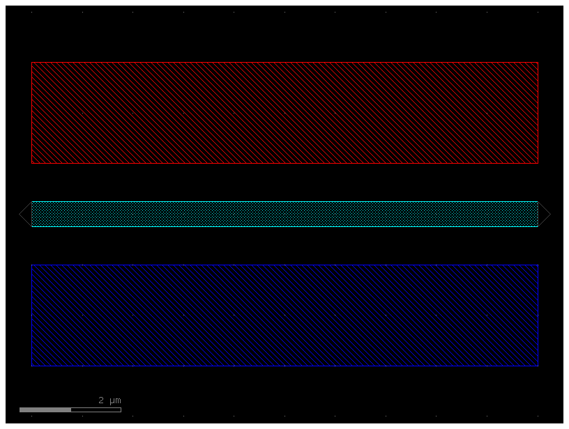
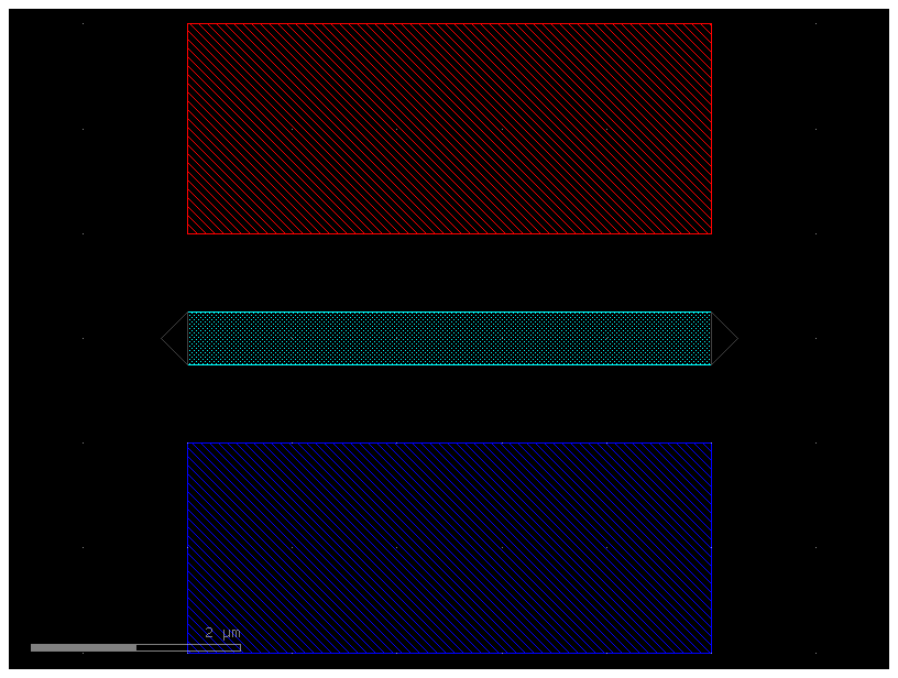
Let’s start off by creating two cross-sections we want to transition between. Note we give all the cross-sectional elements names by specifying the name argument in the add() function – this is important because the transition function will try to match names between the two input cross-sections, and any names not present in both inputs will be skipped.

# Create our first CrossSection
import gdsfactory as gf

s0 = gf.Section(width=1.2, offset=0, layer=(2, 0), name="core", port_names=("o1", "o2"))
s1 = gf.Section(width=2.2, offset=0, layer=(3, 0), name="etch")
s2 = gf.Section(width=1.1, offset=3, layer=(1, 0), name="wg2")
X1 = gf.CrossSection(sections=[s0, s1, s2])

# Create the second CrossSection that we want to transition to
s0 = gf.Section(width=1, offset=0, layer=(2, 0), name="core", port_names=("o1", "o2"))
s1 = gf.Section(width=3.5, offset=0, layer=(3, 0), name="etch")
s2 = gf.Section(width=3, offset=5, layer=(1, 0), name="wg2")
X2 = gf.CrossSection(sections=[s0, s1, s2])

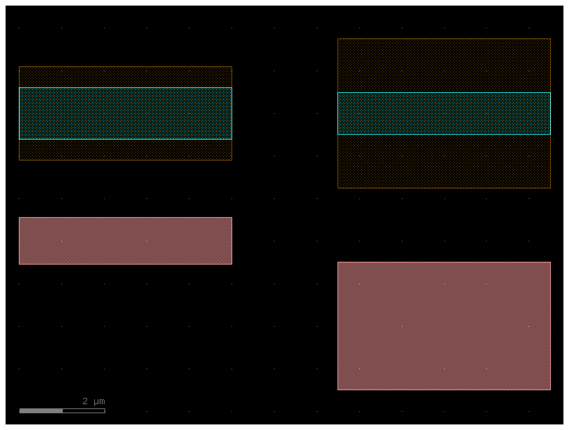
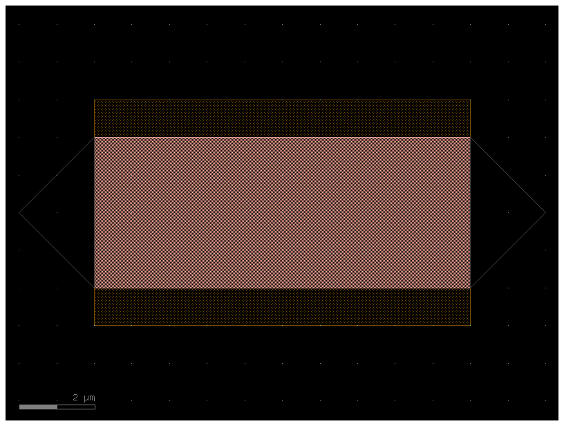
# To show the cross-sections, let's create two Paths and
# create Components by extruding them
P1 = gf.path.straight(length=5)
P2 = gf.path.straight(length=5)
wg1 = gf.path.extrude(P1, X1)
wg2 = gf.path.extrude(P2, X2)

# Place both cross-section Components and quickplot them
c = gf.Component("demo")
wg1ref = c << wg1
wg2ref = c << wg2
wg2ref.movex(7.5)

c.plot()

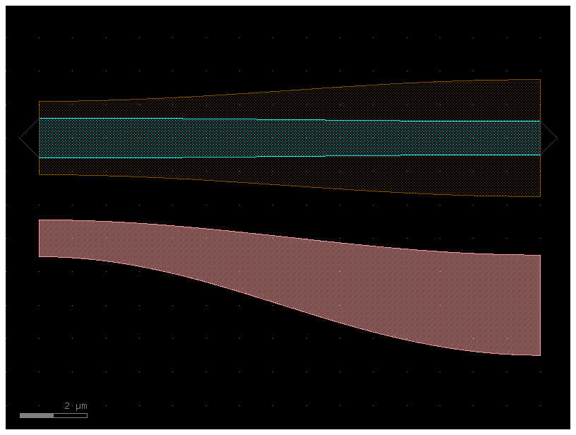
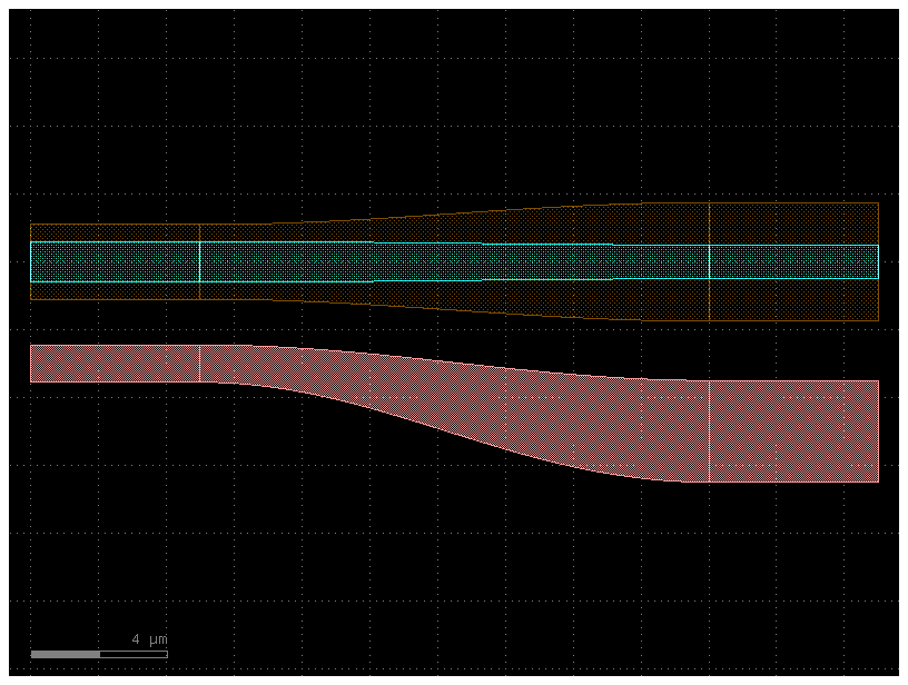
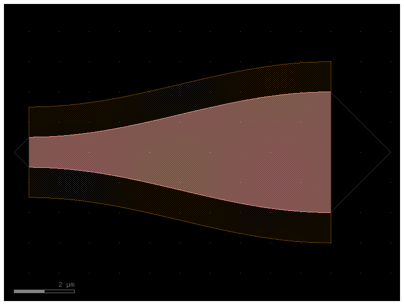
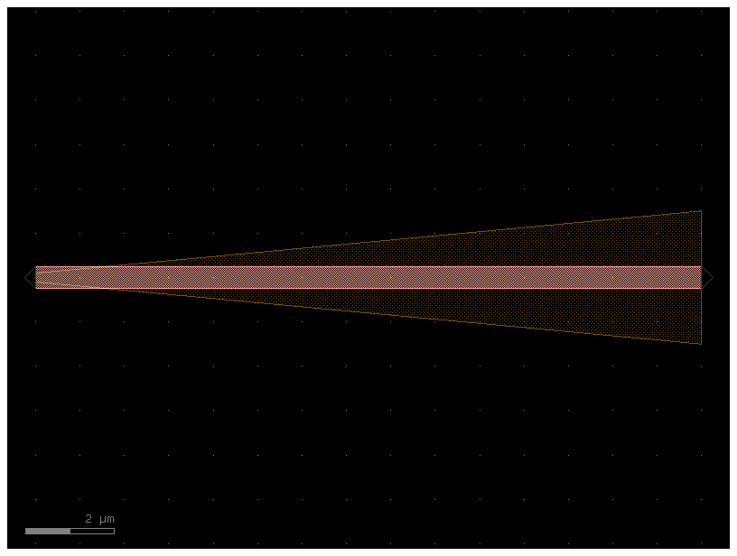
../_images/557eaf27a0603cd9312cd9f0705a56d4c851c8222c16e8c33535b2e8ae383902.png

Now let’s create the transitional CrossSection by calling transition() with these two CrossSections as input. If we want the width to vary as a smooth sinusoid between the sections, we can set width_type to 'sine' (alternatively we could also use 'linear').

# Create the transitional CrossSection
Xtrans = gf.path.transition(cross_section1=X1, cross_section2=X2, width_type="sine")

# Create a Path for the transitional CrossSection to follow
P3 = gf.path.straight(length=15, npoints=100)

# Use the transitional CrossSection to create a Component
straight_transition = gf.path.extrude_transition(P3, Xtrans)
straight_transition.plot()

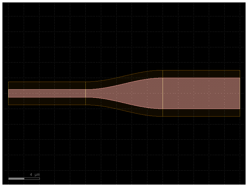
../_images/815326367473313ffe811168657d368d006060f99a6b36ad4e49d33de32f2c0a.png

Now that we have all of our components, let’s connect() everything and see what it looks like

c = gf.Component("transition_demo")

wg1ref = c << wg1
wgtref = c << straight_transition
wg2ref = c << wg2

wgtref.connect("o1", wg1ref.ports["o2"])
wg2ref.connect("o1", wgtref.ports["o2"])

c.plot()

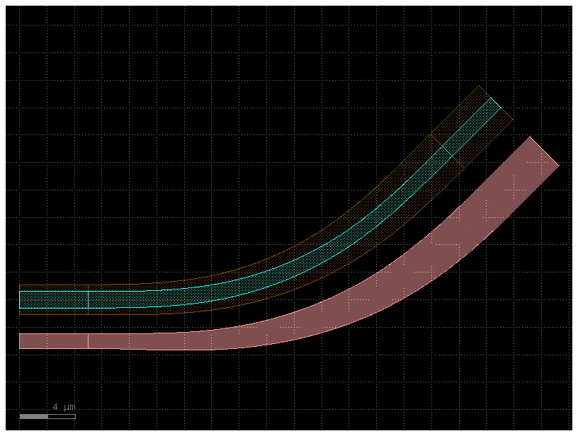
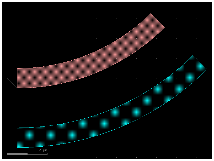
../_images/7b9b76eef7f68f61ebd9525280e12661789eb271a148a5c2facde149d4f62e3a.png

Note that since transition() outputs a Transition, we can make the transition follow an arbitrary path:

# Transition along a curving Path
P4 = gf.path.euler(radius=25, angle=45, p=0.5, use_eff=False)
wg_trans = gf.path.extrude_transition(P4, Xtrans)

c = gf.Component("demo_transition")
wg1_ref = c << wg1  # First cross-section Component
wg2_ref = c << wg2
wgt_ref = c << wg_trans

wgt_ref.connect("o1", wg1_ref.ports["o2"])
wg2_ref.connect("o1", wgt_ref.ports["o2"])

c.plot()

2025-01-19 23:48:31.628 | WARNING  | gdsfactory.component:_write_library:1934 - UserWarning: Component demo_transition has invalid transformations. Try component.flatten_offgrid_references() first.

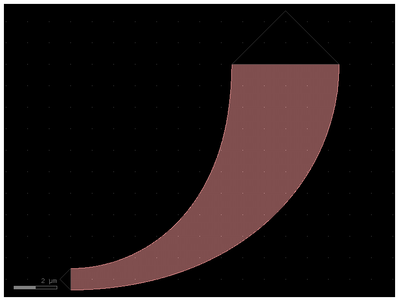
../_images/abc3a107d5983054baf378ad7088941c5be5a867778b25086384070d03908fda.png

Since a Transition inherits from CrossSection you can also extrude an arbitrary Transition.

Extruding a Path

w1 = 1
w2 = 5
x1 = gf.get_cross_section("xs_sc", width=w1)
x2 = gf.get_cross_section("xs_sc", width=w2)
transition = gf.path.transition(x1, x2)
p = gf.path.arc(radius=10)
c = gf.path.extrude(p, transition)
c.plot()

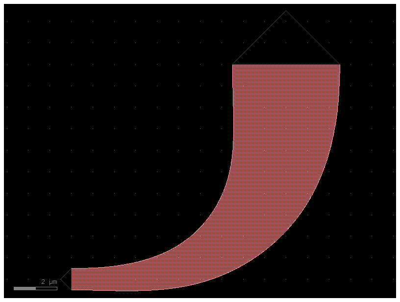
../_images/11ea77426f877135b83c39b8497d107731683775372ece26a997b604bedfd16f.png

Or as a CrossSection for a component

w1 = 1
w2 = 5
length = 10
x1 = gf.get_cross_section("xs_sc", width=w1)
x2 = gf.get_cross_section("xs_sc", width=w2)
transition = gf.path.transition(x1, x2)
c = gf.components.bend_euler(radius=10, cross_section=transition)
c.plot()

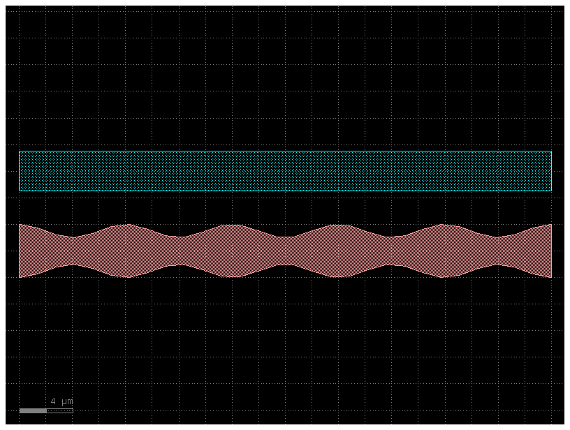
../_images/66bc4753ff37d0e366102c622ff120c5516d34db36b715cd60f2a13639505532.png

Variable width / offset#

In some instances, you may want to vary the width or offset of the path’s cross- section as it travels. This can be accomplished by giving the CrossSection arguments that are functions or lists. Let’s say we wanted a width that varies sinusoidally along the length of the Path. To do this, we need to make a width function that is parameterized from 0 to 1: for an example function my_width_fun(t) where the width at t==0 is the width at the beginning of the Path and the width at t==1 is the width at the end.

import numpy as np
import gdsfactory as gf


def my_custom_width_fun(t):
    # Note: Custom width/offset functions MUST be vectorizable--you must be able
    # to call them with an array input like my_custom_width_fun([0, 0.1, 0.2, 0.3, 0.4])
    num_periods = 5
    return 3 + np.cos(2 * np.pi * t * num_periods)


# Create the Path
P = gf.path.straight(length=40, npoints=30)

# Create two cross-sections: one fixed width, one modulated by my_custom_offset_fun
s0 = gf.Section(width=3, offset=-6, layer=(2, 0))
s1 = gf.Section(width=0, width_function=my_custom_width_fun, offset=0, layer=(1, 0))
X = gf.CrossSection(sections=[s0, s1])

# Extrude the Path to create the Component
c = gf.path.extrude(P, cross_section=X)
c.plot()

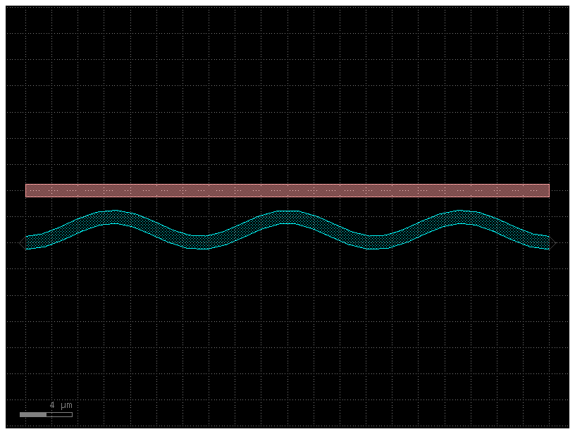
../_images/42a34d2a08dd613fe1ce78c92fbcd56c35be61e00381b6faa9eb6c15e2fec769.png

We can do the same thing with the offset argument:

def my_custom_offset_fun(t):
    # Note: Custom width/offset functions MUST be vectorizable--you must be able
    # to call them with an array input like my_custom_offset_fun([0, 0.1, 0.2, 0.3, 0.4])
    num_periods = 3
    return 3 + np.cos(2 * np.pi * t * num_periods)


# Create the Path
P = gf.path.straight(length=40, npoints=30)

# Create two cross-sections: one fixed offset, one modulated by my_custom_offset_fun
s0 = gf.Section(width=1, offset=0, layer=(1, 0))
s1 = gf.Section(
    width=1,
    offset_function=my_custom_offset_fun,
    layer=(2, 0),
    port_names=["clad1", "clad2"],
)
X = gf.CrossSection(sections=[s0, s1])

# Extrude the Path to create the Component
c = gf.path.extrude(P, cross_section=X)
c.plot()

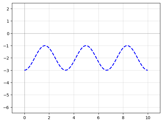
../_images/ee99f57b681cf862308a092ccd4bcde386f5e6dbeac34a4291671f0cd14b1ff8.png

Offsetting a Path#

Sometimes it’s convenient to start with a simple Path and offset the line it follows to suit your needs (without using a custom-offset CrossSection). Here, we start with two copies of simple straight Path and use the offset() function to directly modify each Path.

def my_custom_offset_fun(t):
    # Note: Custom width/offset functions MUST be vectorizable--you must be able
    # to call them with an array input like my_custom_offset_fun([0, 0.1, 0.2, 0.3, 0.4])
    num_periods = 3
    return 2 + np.cos(2 * np.pi * t * num_periods)


P1 = gf.path.straight(npoints=101)
P1.offset(offset=my_custom_offset_fun)
f = P1.plot()

Ignoring fixed y limits to fulfill fixed data aspect with adjustable data limits.

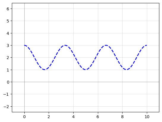
../_images/67bf5c1f8424c451ed64a9fd3b3609e8dea798ed703678d3707c94830496fced.png

P2 = P1.copy()  # Make a copy of the Path
P2.mirror((1, 0))  # reflect across X-axis
f2 = P2.plot()

Ignoring fixed y limits to fulfill fixed data aspect with adjustable data limits.

../_images/57da7f072d3adc2a506afc957dc00b97d4a84039da002f58740f4f39bce7c5b6.png

# Create the Path
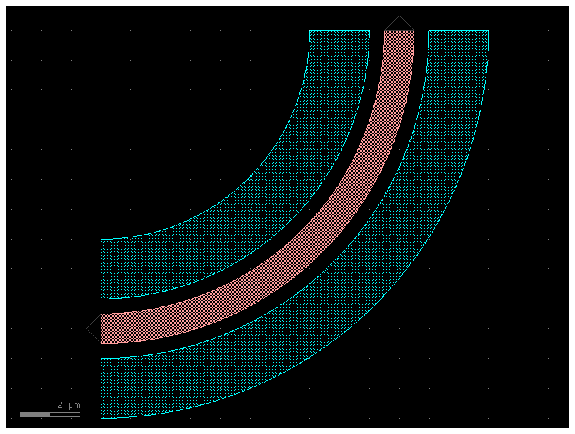
P = gf.path.arc(radius=10, angle=45)

# Create two cross-sections: one fixed width, one modulated by my_custom_offset_fun
s0 = gf.Section(width=1, offset=3, layer=(2, 0), name="waveguide")
s1 = gf.Section(width=1, offset=0, layer=(1, 0), name="heater", port_names=("o1", "o2"))
X = gf.CrossSection(sections=(s0, s1))
c = gf.path.extrude(P, X)
c.plot()

../_images/2c5e1232a4feac36e30fef8c95c95aacaef095c3ff3bab009c598638c2cc98fb.png

P = gf.Path()
P.append(gf.path.arc(radius=10, angle=90))  # Circular arc
P.append(gf.path.straight(length=10))  # Straight section
P.append(gf.path.euler(radius=3, angle=-90))  # Euler bend (aka "racetrack" curve)
P.append(gf.path.straight(length=40))
P.append(gf.path.arc(radius=8, angle=-45))
P.append(gf.path.straight(length=10))
P.append(gf.path.arc(radius=8, angle=45))
P.append(gf.path.straight(length=10))

f = P.plot()

Ignoring fixed y limits to fulfill fixed data aspect with adjustable data limits.

c = gf.path.extrude(P, width=1, layer=(2, 0))
c.plot()

../_images/0781c3a7eec784201a7966e653e9a6d53a0250429d41f0bd34b8aade8f1d4720.png

s0 = gf.Section(width=2, offset=0, layer=(2, 0))
xs = gf.CrossSection(sections=(s0,))
c = gf.path.extrude(P, xs)
c.plot()

../_images/be3016704d0d9c760a1503dceb03448644ca6428e32b40ba054d108589085278.png

p = gf.path.straight(length=10, npoints=101)
s0 = gf.Section(width=1, offset=0, layer=(1, 0), port_names=("o1", "o2"))
s1 = gf.Section(width=3, offset=0, layer=(3, 0))
x1 = gf.CrossSection(sections=(s0, s1))
c = gf.path.extrude(p, x1)
c.plot()

../_images/dc8b65ba058e58d55ba7f680382bd6abdc6abd00694790c35c3796c4b783bf63.png

s0 = gf.Section(width=1 + 3, offset=0, layer=(1, 0), port_names=("o1", "o2"))
s1 = gf.Section(width=3 + 3, offset=0, layer=(3, 0))
x2 = gf.CrossSection(sections=(s0, s1))
c2 = gf.path.extrude(p, x2)
c2.plot()

../_images/d0756443590737ac7a01b2625127b4f9c04066eeb4469da4a6fb824ee651e189.png

t = gf.path.transition(x1, x2)
c3 = gf.path.extrude_transition(p, t)
c3.plot()

../_images/c894dfb19ebe3298dac346706482f94b23fe37698e35b6a0cdcb32e468c920cb.png

c4 = gf.Component("demo_transition2")
start_ref = c4 << c
trans_ref = c4 << c3
end_ref = c4 << c2

trans_ref.connect("o1", start_ref.ports["o2"])
end_ref.connect("o1", trans_ref.ports["o2"])
c4.plot()

../_images/24bdda97c470f6b58626af75b24c501c276256111402c19d677d3d274c8f158d.png

Creating new cross_sections#

You can create functions that return a cross_section in 2 ways:

Customize an existing cross-section for example gf.cross_section.strip
Define a function that returns a cross_section
Define a CrossSection object

What parameters do cross_section take?

help(gf.cross_section.cross_section)

Help on function cross_section in module gdsfactory.cross_section:

cross_section(width: 'float' = 0.5, offset: 'float' = 0, layer: 'LayerSpec | None' = 'WG', sections: 'tuple[Section, ...] | None' = None, port_names: 'tuple[str, str]' = ('o1', 'o2'), port_types: 'tuple[str, str]' = ('optical', 'optical'), bbox_layers: 'LayerSpecs | None' = None, bbox_offsets: 'Floats | None' = None, cladding_layers: 'LayerSpecs | None' = None, cladding_offsets: 'Floats | None' = None, cladding_simplify: 'Floats | None' = None, radius: 'float | None' = 10.0, radius_min: 'float | None' = None, main_section_name: 'str' = '_default', **kwargs) -> 'CrossSection'
    Return CrossSection.

    Args:
        width: main Section width (um).
        offset: main Section center offset (um).
        layer: main section layer.
        sections: list of Sections(width, offset, layer, ports).
        port_names: for input and output ('o1', 'o2').
        port_types: for input and output: electrical, optical, vertical_te ...
        bbox_layers: list of layers bounding boxes to extrude.
        bbox_offsets: list of offset from bounding box edge.
        cladding_layers: list of layers to extrude.
        cladding_offsets: list of offset from main Section edge.
        cladding_simplify: Optional Tolerance value for the simplification algorithm.                 All points that can be removed without changing the resulting.                 polygon by more than the value listed here will be removed.
        radius: routing bend radius (um).
        radius_min: min acceptable bend radius.
        main_section_name: name of the main section. Defaults to _default

    .. plot::
        :include-source:

        import gdsfactory as gf

        xs = gf.cross_section.cross_section(width=0.5, offset=0, layer='WG')
        p = gf.path.arc(radius=10, angle=45)
        c = p.extrude(xs)
        c.plot()

    .. code::


           ┌────────────────────────────────────────────────────────────┐
           │                                                            │
           │                                                            │
           │                   boox_layer                               │
           │                                                            │
           │         ┌──────────────────────────────────────┐           │
           │         │                            ▲         │bbox_offset│
           │         │                            │         ├──────────►│
           │         │           cladding_offset  │         │           │
           │         │                            │         │           │
           │         ├─────────────────────────▲──┴─────────┤           │
           │         │                         │            │           │
        ─ ─┤         │           core   width  │            │           ├─ ─ center
           │         │                         │            │           │
           │         ├─────────────────────────▼────────────┤           │
           │         │                                      │           │
           │         │                                      │           │
           │         │                                      │           │
           │         │                                      │           │
           │         └──────────────────────────────────────┘           │
           │                                                            │
           │                                                            │
           │                                                            │
           └────────────────────────────────────────────────────────────┘

from functools import partial
import gdsfactory as gf

pin = partial(
    gf.cross_section.strip,
    layer=(2, 0),
    sections=(
        gf.Section(layer=(21, 0), width=2, offset=+2),
        gf.Section(layer=(20, 0), width=2, offset=-2),
    ),
)

c = gf.components.straight(cross_section=pin)
c.plot()

../_images/170a9079b96f239cffa919982c1d34c883a707bbbc517c43f66f80ccd7fa24ce.png

pin5 = gf.components.straight(cross_section=pin, length=5)
pin5.plot()

../_images/e589ef4f65883b4dd0bad80fe6a9c79ad88a4f3ea1e3ecf0f10722f673c516dc.png

finally, you can also pass most components Dict that define the cross-section

# Create our first CrossSection
s0 = gf.Section(width=0.5, offset=0, layer=(1, 0), name="wg", port_names=("o1", "o2"))
s1 = gf.Section(width=0.2, offset=0, layer=(3, 0), name="slab")
x1 = gf.CrossSection(sections=(s0, s1))

# Create the second CrossSection that we want to transition to
s0 = gf.Section(width=0.5, offset=0, layer=(1, 0), name="wg", port_names=("o1", "o2"))
s1 = gf.Section(width=3.0, offset=0, layer=(3, 0), name="slab")
x2 = gf.CrossSection(sections=(s0, s1))

# To show the cross-sections, let's create two Paths and create Components by extruding them
p1 = gf.path.straight(length=5)
p2 = gf.path.straight(length=5)
wg1 = gf.path.extrude(p1, x1)
wg2 = gf.path.extrude(p2, x2)

# Place both cross-section Components and quickplot them
c = gf.Component()
wg1ref = c << wg1
wg2ref = c << wg2
wg2ref.movex(7.5)

# Create the transitional CrossSection
xtrans = gf.path.transition(cross_section1=x1, cross_section2=x2, width_type="linear")
# Create a Path for the transitional CrossSection to follow
p3 = gf.path.straight(length=15, npoints=100)

# Use the transitional CrossSection to create a Component
straight_transition = gf.path.extrude_transition(p3, xtrans)
straight_transition.plot()

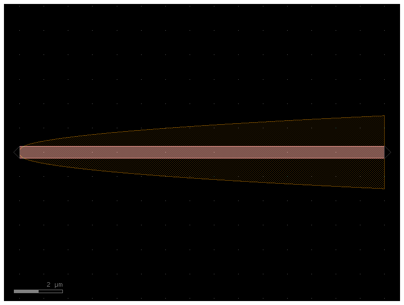
../_images/4b229558ea4e1979c38c43fcd777ee7f3143ad81f41715605afbe19f587665e1.png

# Create the transitional CrossSection
xtrans = gf.path.transition(
    cross_section1=x1, cross_section2=x2, width_type="parabolic"
)
# Create a Path for the transitional CrossSection to follow
p3 = gf.path.straight(length=15, npoints=100)

# Use the transitional CrossSection to create a Component
straight_transition = gf.path.extrude_transition(p3, xtrans)
straight_transition.plot()

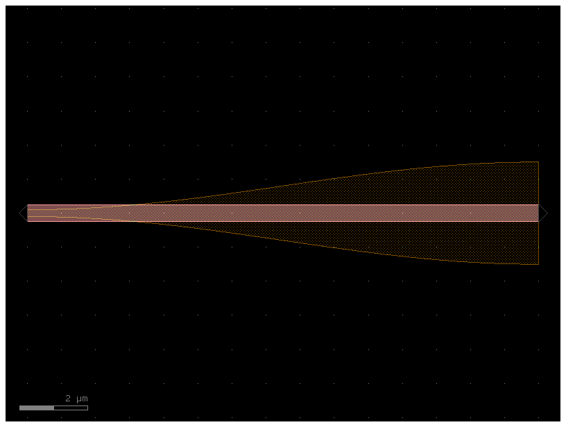
../_images/99e3c10ee0498abbbaa501a5e03d2835dafe61ad7175fc41b460de4403b6f88b.png

# Create the transitional CrossSection
xtrans = gf.path.transition(cross_section1=x1, cross_section2=x2, width_type="sine")
# Create a Path for the transitional CrossSection to follow
p3 = gf.path.straight(length=15, npoints=100)

# Use the transitional CrossSection to create a Component
straight_transition = gf.path.extrude_transition(p3, xtrans)
straight_transition.plot()

../_images/0c33d699a1a44aa03ede9b7cb65b02a55abca31f62764d082ee9d9bdfca07012.png

s = straight_transition.to_3d()
s.show()

Waveguides with Shear Faces#

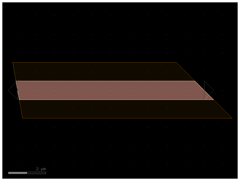
By default, an extruded path will end in a face orthogonal to the direction of the path. Sometimes you want to have a sheared face that tilts at a given angle from this orthogonal baseline. You can supply the parameters shear_angle_start and shear_angle_end to the extrude() function.

P = gf.path.straight(length=10)

s0 = gf.Section(width=1, offset=0, layer=(1, 0), port_names=("o1", "o2"))
s1 = gf.Section(width=3, offset=0, layer=(3, 0))
X1 = gf.CrossSection(sections=(s0, s1))
c = gf.path.extrude(P, X1, shear_angle_start=10, shear_angle_end=45)
c.plot()

../_images/1b24372b1e56ae0623b4cb114ac03665d5073bae79009b3bab0819f15cb527a8.png

c.pprint_ports()

┏━━━━━━┳━━━━━━━┳━━━━━━━━━━━━━┳━━━━━━━━━━━━━┳━━━━━━━━┳━━━━━━━━━━━┳━━━━━━━━━━━━━┓
┃ name ┃ width ┃ center      ┃ orientation ┃ layer  ┃ port_type ┃ shear_angle ┃
┡━━━━━━╇━━━━━━━╇━━━━━━━━━━━━━╇━━━━━━━━━━━━━╇━━━━━━━━╇━━━━━━━━━━━╇━━━━━━━━━━━━━┩
│ o1   │ 1.0   │ [0.0, 0.0]  │ 180         │ [1, 0] │ optical   │ 10          │
│ o2   │ 1.0   │ [10.0, 0.0] │ 0.0         │ [1, 0] │ optical   │ 45          │
└──────┴───────┴─────────────┴─────────────┴────────┴───────────┴─────────────┘

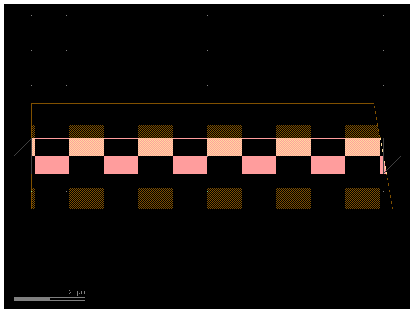
By default, the shear angle parameters are None, in which case shearing will not be applied to the face.

c = gf.path.extrude(P, X1, shear_angle_start=None, shear_angle_end=10)
c.plot()

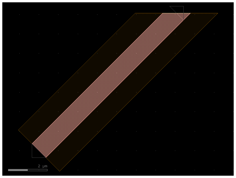
../_images/c5dd36a2ea7f36a47e8b397f0531e93d9c1561ee8178ad9f77d0ec607095924c.png

Shearing should work on paths of arbitrary orientation, as long as their end segments are sufficiently long.

angle = 45
P = gf.path.straight(length=10).rotate(angle)
c = gf.path.extrude(P, X1, shear_angle_start=angle, shear_angle_end=angle)
c.plot()

../_images/e864e98170b5eaa5d290f94b0710f44e1a1992df4a92adf5fd455cf5dd5fef6e.png

For a non-linear path or width profile, the algorithm will intersect the path when sheared inwards and extrapolate linearly going outwards.

angle = 15
P = gf.path.euler()
c = gf.path.extrude(P, X1, shear_angle_start=angle, shear_angle_end=angle)
c.plot()

../_images/e1924482986e7f0f5b7118205bc17b93ac28ca1cdb5ac80ead5188a46eb4a724.png

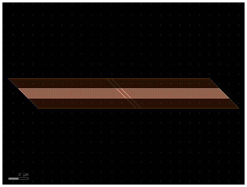
The port location, width and orientation remains the same for a sheared component. However, an additional property, shear_angle is set to the value of the shear angle. In general, shear ports can be safely connected together.

p1 = gf.path.straight(length=10)
p2 = gf.path.straight(length=0.5)
s0 = gf.Section(width=1, offset=0, layer=(1, 0), port_names=("o1", "o2"))
s1 = gf.Section(width=3, offset=0, layer=(3, 0))
xs = gf.CrossSection(sections=(s0, s1))

c1 = gf.path.extrude(p1, xs, shear_angle_start=45, shear_angle_end=45)
c2 = gf.path.extrude(p2, xs, shear_angle_start=45, shear_angle_end=45)

c = gf.Component("shear_sample")
ref1 = c << c1
ref2 = c << c2
ref3 = c << c1


ref1.connect(port="o1", destination=ref2.ports["o1"])
ref3.connect(port="o1", destination=ref2.ports["o2"])
c.plot()

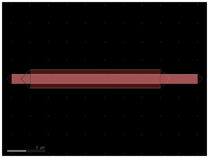
../_images/2c5e08bab130b9328d491d7fe8fd6fac00fcd434bfdbebd7ef9532bd40cf9173.png

Transitions with Shear faces#

You can also create a transition with a shear face

P = gf.path.straight(length=10)

s0 = gf.Section(width=1, offset=0, layer=(1, 0), name="core", port_names=("o1", "o2"))
s1 = gf.Section(width=3, offset=0, layer=(3, 0), name="slab")
X1 = gf.CrossSection(sections=(s0, s1))

s2 = gf.Section(width=0.5, offset=0, layer=(1, 0), name="core", port_names=("o1", "o2"))
s3 = gf.Section(width=2.0, offset=0, layer=(3, 0), name="slab")
X2 = gf.CrossSection(sections=(s2, s3))
t = gf.path.transition(X1, X2, width_type="linear")
c = gf.path.extrude_transition(P, t, shear_angle_start=10, shear_angle_end=45)
c.plot()

../_images/6a08b2343bb14699c75e7cc7b594d5736f37088b4d3b580dee2dc256077b62b8.png

This will also work with curves and non-linear width profiles. Keep in mind that points outside the original geometry will be extrapolated linearly.

angle = 15
P = gf.path.euler()
c = gf.path.extrude_transition(P, t, shear_angle_start=angle, shear_angle_end=angle)
c.plot()

../_images/5a62967ee117e1090553abe4a7ffb73af21f073b364c6d2a4aaf65800454487f.png

bbox_layers vs cladding_layers#

For extruding waveguides you have two options:

bbox_layers for squared bounding box
cladding_layers for extruding a layer that follows the shape of the path.

xs_bbox = gf.cross_section.cross_section(bbox_layers=[(3, 0)], bbox_offsets=[3])
w1 = gf.components.bend_euler(cross_section=xs_bbox)
w1.plot()

../_images/3cb903cd561c44a029b1eec5068c31635cda9a3058c9b3254e4892076f5a9884.png

xs_clad = gf.cross_section.cross_section(cladding_layers=[(3, 0)], cladding_offsets=[3])
w2 = gf.components.bend_euler(cross_section=xs_clad)
w2.plot()

../_images/3c53aae8d5a9749f066ef8b40878f5807819192c35e70d8883b3b420a96f402c.png

Insets#

It’s handy to be able to extrude a CrossSection along a Path, while each Section may have a particular inset relative to the main Section. An example of this is a waveguide with a heater.

import gdsfactory as gf


def xs_waveguide_heater() -> gf.CrossSection:
    return gf.cross_section.cross_section(
        layer="WG",
        width=0.5,
        sections=(
            gf.cross_section.Section(
                name="heater",
                width=1,
                layer="HEATER",
                insets=(1, 2),
            ),
        ),
    )


c = gf.components.straight(cross_section=xs_waveguide_heater)
c.plot()

../_images/b843f6afd644e42b257dcc59df0cf5fd2868be9f78f40ff776a4112f3031e814.png

def xs_waveguide_heater_with_ports() -> gf.CrossSection:
    return gf.cross_section.cross_section(
        layer="WG",
        width=0.5,
        sections=(
            gf.cross_section.Section(
                name="heater",
                width=1,
                layer="HEATER",
                insets=(1, 2),
                port_names=("e1", "e2"),
                port_types=("electrical", "electrical"),
            ),
        ),
    )


c = gf.components.straight(cross_section=xs_waveguide_heater_with_ports)
c.plot()

../_images/607906dbd042c86a6b8d07d9980aea7c6c3d13b6487d762b5286181f1792db73.png

Path and CrossSection

Contents

Path and CrossSection#

Path#

CrossSection#

Option 1: Single layer and width cross-section#

Option 2: Arbitrary Cross-section#

Option 3: CrossSection with ComponentAlongPath#

Path#

Waypoint smooth paths#

Waypoint sharp paths#

Custom curves#

Simplifying / reducing point usage#

Curvature calculation#

Transitioning between cross-sections#

Variable width / offset#

Offsetting a Path#

Creating new cross_sections#

Waveguides with Shear Faces#

Transitions with Shear faces#

bbox_layers vs cladding_layers#

Insets#