CPW length sweep and de-embedding
Simulate 100, 400, and 800 µm CPW lines with both lumped ports and wave ports over 300 frequencies from 1 to 100 GHz. De-embed the 100 µm reference from each longer line and compare propagation, impedance, and distributed RLGC parameters. Then check the cross-section modes and voltage–power impedance with a 2D eigensolver at 10, 25, 50, 75, and 100 GHz, and use that impedance to turn the de-embedded propagation constant into physical R, L, G, and C.
Start with the basic lumped-port or wave-port example for a single simulation. This notebook is self-contained and runs both sweeps when executed from top to bottom.
Requirements:
- IHP PDK:
uv pip install ihp-gdsfactory - scikit-rf:
uv pip install scikit-rf - GDSFactory+ account for cloud simulation
Define the CPW
import gdsfactory as gf
from ihp import LAYER, PDK

PDK.activate()


@gf.cell
def gsg_electrode(
    length: float = 800,
    s_width: float = 20,
    g_width: float = 40,
    gap_width: float = 15,
    layer=LAYER.TopMetal2drawing,
) -> gf.Component:
    """
    Create a GSG (Ground-Signal-Ground) electrode.

    Args:
        length: horizontal length of the electrodes
        s_width: width of the signal (center) electrode
        g_width: width of the ground electrodes
        gap_width: gap between signal and ground electrodes
        layer: layer for the metal
    """
    c = gf.Component()

    r1 = c << gf.c.rectangle((length, g_width), centered=True, layer=layer)
    r1.move((0, (g_width + s_width) / 2 + gap_width))

    _r2 = c << gf.c.rectangle((length, s_width), centered=True, layer=layer)

    r3 = c << gf.c.rectangle((length, g_width), centered=True, layer=layer)
    r3.move((0, -(g_width + s_width) / 2 - gap_width))

    c.add_port(
        name="o1",
        center=(-length / 2, 0),
        width=s_width,
        orientation=180,
        port_type="electrical",
        layer=layer,
    )

    c.add_port(
        name="o2",
        center=(length / 2, 0),
        width=s_width,
        orientation=0,
        port_type="electrical",
        layer=layer,
    )

    return c


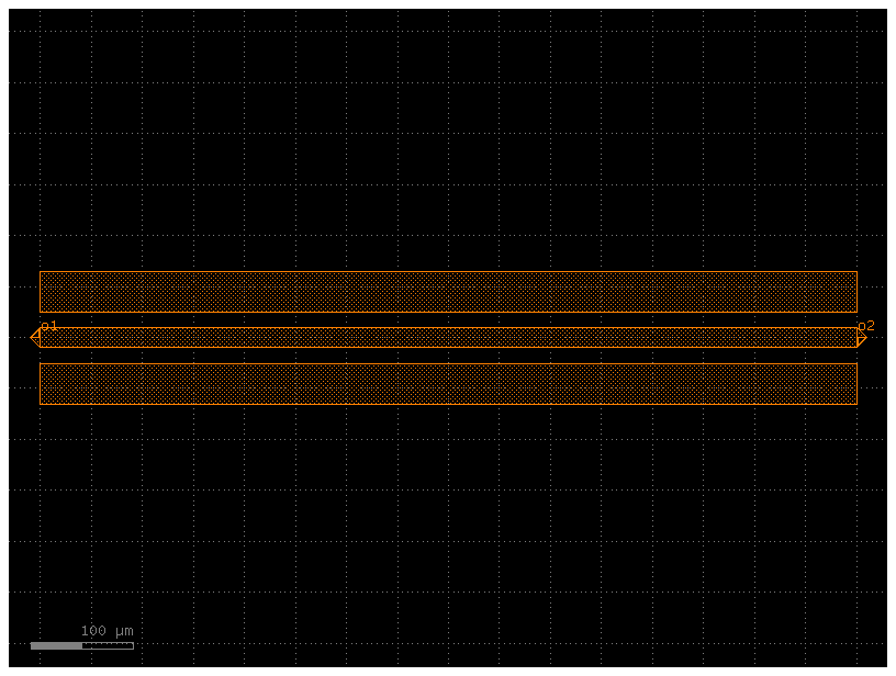
c = gsg_electrode()
cc = c.copy()
cc.draw_ports()
cc
Configure both port types
Use the geometry, materials, airbox, and solver settings from the basic examples. Both ports are excited in separate solves to obtain all four S-parameters required for de-embedding.
The examples use different airbox margins for the two port types. The study checks length consistency within each setup; a physical comparison between port types also requires airbox and mesh convergence.
from gsim.common.stack import get_stack
from gsim.palace import DrivenSim


def setup_sim(cell, port_type, *, solver_type="Default"):
    sim = DrivenSim()
    if port_type == "lumped":
        output_name = "lumped"
    elif port_type == "wave":
        output_name = f"waveport-{solver_type.lower()}"
    else:
        raise ValueError(f"Unknown port type: {port_type}")
    sim.set_output_dir(f"./palace-sim-cpw-{output_name}-{cell.name}")
    sim.set_geometry(cell)
    sim.set_stack(get_stack())

    if port_type == "lumped":
        sim.set_airbox(margin_x=50, margin_y=0, z_above=100, z_below=100)
        for port_name in ["o1", "o2"]:
            sim.add_cpw_port(
                port_name, layer="topmetal2", s_width=20, gap_width=15, excited=True
            )
    else:
        sim.set_airbox(margin_x=0.0, margin_y=50, z_above=100.0, z_below=100.0)
        for port_name in ["o1", "o2"]:
            sim.add_wave_port(
                port_name,
                layer="topmetal2",
                max_size=True,
                mode=1,
                excited=True,
                eigensolver_type=solver_type,
                eigensolver_tol=1e-6,
                eigensolver_ksp_tol=1e-8,
                eigensolver_max_size=40,
                eigensolver_verbose=0,
            )

    sim.set_driven(fmin=1e9, fmax=100e9, num_points=300)
    print(sim.validate_config())
    return sim
Run the length sweep
Run all six cases, reusing matching cached results, including the 800 µm simulations from the basic notebooks. Submit the jobs without waiting, then collect their results in the same order.
Lumped-port validation reads the mesh once per gap surface: two ports × two gaps gives four reads before the cache lookup. Extracting results.tar.gz... means downloaded results are being unpacked, including on cache hits. Use verbose="full" instead of "status" if you need solver logs.
lengths_um = (100, 400, 800)
port_types = ("lumped", "wave")
port_labels = {"lumped": "Lumped ports", "wave": "Wave ports"}
job_ids = {}

for port_type in port_types:
    for length_um in lengths_um:
        component = gsg_electrode(length=length_um)
        simulation = setup_sim(component, port_type)
        simulation.mesh(
            preset="default",
            refined_mesh_size=2.0,
            max_mesh_size=40.0,
            fmax=150e9,
            verbose=False,
        )
        job_ids[port_type, length_um] = simulation.run(
            wait=False, check_cache=True, verbose="status"
        )
Validation: PASSED


Info    : Reading 'palace-sim-cpw-lumped-gsg_electrode_L100_SW20_GW40_GW15_LTopMetal2drawing/palace.msh'...
Info    : 5800 nodes
Info    : 41496 elements
Info    : Done reading 'palace-sim-cpw-lumped-gsg_electrode_L100_SW20_GW40_GW15_LTopMetal2drawing/palace.msh'
Info    : Reading 'palace-sim-cpw-lumped-gsg_electrode_L100_SW20_GW40_GW15_LTopMetal2drawing/palace.msh'...
Info    : 5800 nodes
Info    : 41496 elements
Info    : Done reading 'palace-sim-cpw-lumped-gsg_electrode_L100_SW20_GW40_GW15_LTopMetal2drawing/palace.msh'
Info    : Reading 'palace-sim-cpw-lumped-gsg_electrode_L100_SW20_GW40_GW15_LTopMetal2drawing/palace.msh'...
Info    : 5800 nodes
Info    : 41496 elements
Info    : Done reading 'palace-sim-cpw-lumped-gsg_electrode_L100_SW20_GW40_GW15_LTopMetal2drawing/palace.msh'
Info    : Reading 'palace-sim-cpw-lumped-gsg_electrode_L100_SW20_GW40_GW15_LTopMetal2drawing/palace.msh'...
Info    : 5800 nodes
Info    : 41496 elements
Info    : Done reading 'palace-sim-cpw-lumped-gsg_electrode_L100_SW20_GW40_GW15_LTopMetal2drawing/palace.msh'
Info    : Reading 'palace-sim-cpw-lumped-gsg_electrode_L100_SW20_GW40_GW15_LTopMetal2drawing/palace.msh'...
Info    : 5800 nodes
Info    : 41496 elements


Info    : Done reading 'palace-sim-cpw-lumped-gsg_electrode_L100_SW20_GW40_GW15_LTopMetal2drawing/palace.msh'


Cache hit: reusing job 01a163df-7f17-72a4-91e9-f92caebbe9aa
Validation: PASSED


Info    : Reading 'palace-sim-cpw-lumped-gsg_electrode_L400_SW20_GW40_GW15_LTopMetal2drawing/palace.msh'...
Info    : 14840 nodes
Info    : 106937 elements
Info    : [  0%] Reading elements
Info : [ 10%] Reading elements
Info : [ 20%] Reading elements
Info : [ 30%] Reading elements
Info : [ 40%] Reading elements
Info : [ 50%] Reading elements
Info : [ 60%] Reading elements
Info : [ 70%] Reading elements
Info : [ 80%] Reading elements
Info : [ 90%] Reading elements
Info : Done reading 'palace-sim-cpw-lumped-gsg_electrode_L400_SW20_GW40_GW15_LTopMetal2drawing/palace.msh'
Info : Reading 'palace-sim-cpw-lumped-gsg_electrode_L400_SW20_GW40_GW15_LTopMetal2drawing/palace.msh'...
Info : 14840 nodes
Info : 106937 elements
Info : [ 0%] Reading elements
Info : [ 10%] Reading elements
Info : [ 20%] Reading elements
Info : [ 30%] Reading elements
Info : [ 40%] Reading elements
Info : [ 50%] Reading elements
Info : [ 60%] Reading elements
Info : [ 70%] Reading elements
Info : [ 80%] Reading elements
Info : [ 90%] Reading elements
Info : Done reading 'palace-sim-cpw-lumped-gsg_electrode_L400_SW20_GW40_GW15_LTopMetal2drawing/palace.msh'
Info : Reading 'palace-sim-cpw-lumped-gsg_electrode_L400_SW20_GW40_GW15_LTopMetal2drawing/palace.msh'...
Info : 14840 nodes
Info : 106937 elements
Info : [ 0%] Reading elements
Info : [ 10%] Reading elements
Info : [ 20%] Reading elements
Info : [ 30%] Reading elements
Info : [ 40%] Reading elements
Info : [ 50%] Reading elements
Info : [ 60%] Reading elements
Info : [ 70%] Reading elements
Info : [ 80%] Reading elements
Info : [ 90%] Reading elements
Info : Done reading 'palace-sim-cpw-lumped-gsg_electrode_L400_SW20_GW40_GW15_LTopMetal2drawing/palace.msh' Info : Reading 'palace-sim-cpw-lumped-gsg_electrode_L400_SW20_GW40_GW15_LTopMetal2drawing/palace.msh'... Info : 14840 nodes Info : 106937 elements Info : [ 0%] Reading elements
Info : [ 10%] Reading elements
Info : [ 20%] Reading elements
Info : [ 30%] Reading elements
Info : [ 40%] Reading elements
Info : [ 50%] Reading elements
Info : [ 60%] Reading elements
Info : [ 70%] Reading elements
Info : [ 80%] Reading elements
Info : [ 90%] Reading elements
Info : Done reading 'palace-sim-cpw-lumped-gsg_electrode_L400_SW20_GW40_GW15_LTopMetal2drawing/palace.msh'
Info : Reading 'palace-sim-cpw-lumped-gsg_electrode_L400_SW20_GW40_GW15_LTopMetal2drawing/palace.msh'...
Info : 14840 nodes
Info : 106937 elements
Info : [ 0%] Reading elements
Info : [ 10%] Reading elements
Info : [ 20%] Reading elements
Info : [ 30%] Reading elements
Info : [ 40%] Reading elements
Info : [ 50%] Reading elements
Info : [ 60%] Reading elements
Info : [ 70%] Reading elements
Info : [ 80%] Reading elements
Info : [ 90%] Reading elements
Info    : Done reading 'palace-sim-cpw-lumped-gsg_electrode_L400_SW20_GW40_GW15_LTopMetal2drawing/palace.msh'


Cache hit: reusing job 01a163e0-2ef6-7391-996d-8b0d8e3843cd
Validation: PASSED


Info    : Reading 'palace-sim-cpw-lumped-gsg_electrode_L800_SW20_GW40_GW15_LTopMetal2drawing/palace.msh'...
Info    : 25428 nodes
Info    : 183685 elements
Info    : [  0%] Reading elements
Info : [ 10%] Reading elements
Info : [ 20%] Reading elements
Info : [ 30%] Reading elements
Info : [ 40%] Reading elements
Info : [ 50%] Reading elements
Info : [ 60%] Reading elements
Info : [ 70%] Reading elements
Info : [ 80%] Reading elements
Info : [ 90%] Reading elements
Info    : Done reading 'palace-sim-cpw-lumped-gsg_electrode_L800_SW20_GW40_GW15_LTopMetal2drawing/palace.msh'
Info    : Reading 'palace-sim-cpw-lumped-gsg_electrode_L800_SW20_GW40_GW15_LTopMetal2drawing/palace.msh'...
Info    : 25428 nodes
Info    : 183685 elements
Info    : [  0%] Reading elements
Info : [ 10%] Reading elements
Info : [ 20%] Reading elements
Info : [ 30%] Reading elements
Info : [ 40%] Reading elements
Info : [ 50%] Reading elements
Info : [ 60%] Reading elements
Info : [ 70%] Reading elements
Info : [ 80%] Reading elements
Info : [ 90%] Reading elements
Info : Done reading 'palace-sim-cpw-lumped-gsg_electrode_L800_SW20_GW40_GW15_LTopMetal2drawing/palace.msh'
Info : Reading 'palace-sim-cpw-lumped-gsg_electrode_L800_SW20_GW40_GW15_LTopMetal2drawing/palace.msh'...
Info : 25428 nodes
Info : 183685 elements
Info : [ 0%] Reading elements
Info : [ 10%] Reading elements
Info : [ 20%] Reading elements
Info : [ 30%] Reading elements
Info : [ 40%] Reading elements
Info : [ 50%] Reading elements
Info : [ 60%] Reading elements
Info : [ 70%] Reading elements
Info : [ 80%] Reading elements
Info : [ 90%] Reading elements
Info : Done reading 'palace-sim-cpw-lumped-gsg_electrode_L800_SW20_GW40_GW15_LTopMetal2drawing/palace.msh'
Info : Reading 'palace-sim-cpw-lumped-gsg_electrode_L800_SW20_GW40_GW15_LTopMetal2drawing/palace.msh'...
Info : 25428 nodes
Info : 183685 elements
Info : [ 0%] Reading elements
Info : [ 10%] Reading elements
Info : [ 20%] Reading elements
Info : [ 30%] Reading elements
Info : [ 40%] Reading elements
Info : [ 50%] Reading elements
Info : [ 60%] Reading elements
Info : [ 70%] Reading elements
Info : [ 80%] Reading elements
Info : [ 90%] Reading elements
Info : Done reading 'palace-sim-cpw-lumped-gsg_electrode_L800_SW20_GW40_GW15_LTopMetal2drawing/palace.msh'
Info : Reading 'palace-sim-cpw-lumped-gsg_electrode_L800_SW20_GW40_GW15_LTopMetal2drawing/palace.msh'...
Info : 25428 nodes
Info : 183685 elements
Info : [ 0%] Reading elements
Info : [ 10%] Reading elements
Info : [ 20%] Reading elements
Info : [ 30%] Reading elements
Info : [ 40%] Reading elements
Info : [ 50%] Reading elements
Info : [ 60%] Reading elements
Info : [ 70%] Reading elements
Info : [ 80%] Reading elements
Info : [ 90%] Reading elements
Info : Done reading 'palace-sim-cpw-lumped-gsg_electrode_L800_SW20_GW40_GW15_LTopMetal2drawing/palace.msh'
Cache hit: reusing job 01a163d1-cead-7795-95e8-a005452906fc
Validation: PASSED


Info    : Reading 'palace-sim-cpw-waveport-default-gsg_electrode_L100_SW20_GW40_GW15_LTopMetal2drawing/palace.msh'...
Info    : 10395 nodes
Info    : 62981 elements
Info    : Done reading 'palace-sim-cpw-waveport-default-gsg_electrode_L100_SW20_GW40_GW15_LTopMetal2drawing/palace.msh'


Cache hit: reusing job 01a163e0-59bf-73d2-8c3f-773dce91a570
Validation: PASSED


Info    : Reading 'palace-sim-cpw-waveport-default-gsg_electrode_L400_SW20_GW40_GW15_LTopMetal2drawing/palace.msh'...
Info    : 22166 nodes
Info    : 150924 elements
Info    : [  0%] Reading elements
Info : [ 10%] Reading elements
Info : [ 20%] Reading elements
Info : [ 30%] Reading elements
Info : [ 40%] Reading elements
Info : [ 50%] Reading elements
Info : [ 60%] Reading elements
Info : [ 70%] Reading elements
Info : [ 80%] Reading elements
Info : [ 90%] Reading elements
Info : Done reading 'palace-sim-cpw-waveport-default-gsg_electrode_L400_SW20_GW40_GW15_LTopMetal2drawing/palace.msh'
Cache hit: reusing job 01a163e0-73c4-75a1-9c6d-8ac91c9883bb
Validation: PASSED


Info    : Reading 'palace-sim-cpw-waveport-default-gsg_electrode_L800_SW20_GW40_GW15_LTopMetal2drawing/palace.msh'...
Info    : 36019 nodes
Info    : 255126 elements
Info    : [  0%] Reading elements
Info : [ 10%] Reading elements
Info : [ 20%] Reading elements
Info : [ 30%] Reading elements
Info : [ 40%] Reading elements
Info : [ 50%] Reading elements
Info : [ 60%] Reading elements
Info : [ 70%] Reading elements
Info : [ 80%] Reading elements
Info : [ 90%] Reading elements
Info : Done reading 'palace-sim-cpw-waveport-default-gsg_electrode_L800_SW20_GW40_GW15_LTopMetal2drawing/palace.msh'
Cache hit: reusing job 01a163cf-343a-7355-b9e3-8932876715fa
import gsim

sweep_results = gsim.wait_for_results(list(job_ids.values()), verbose="status")
results_by_case = dict(zip(job_ids, sweep_results, strict=True))
Waiting for 6 jobs...
  palace-b607c9c8                [####################] 100% complete     elapsed 0m 00s
  palace-0004e35b                [####################] 100% complete     elapsed 0m 00s
  palace-d9397d32                [####################] 100% complete     elapsed 0m 00s
  palace-319e1554                [####################] 100% complete     elapsed 0m 00s
  palace-182c4ad6                [####################] 100% complete     elapsed 0m 00s
  palace-3d3b09a1                [####################] 100% complete     elapsed 0m 00s


Extracting results.tar.gz...
Downloaded 12 files to sim-data-palace-b607c9c8


Extracting results.tar.gz...
Downloaded 12 files to sim-data-palace-0004e35b


Extracting results.tar.gz...
Downloaded 12 files to sim-data-palace-d9397d32


Extracting results.tar.gz...
Downloaded 10 files to sim-data-palace-319e1554


Extracting results.tar.gz...
Downloaded 10 files to sim-data-palace-182c4ad6


Extracting results.tar.gz...
Downloaded 10 files to sim-data-palace-3d3b09a1
Prepare the two-port networks
Check that every result contains the full S-matrix before converting it to scikit-rf.
Impedance reference: the two port types give different S-parameters.
- Lumped ports: S is defined in the real 50 Ω port resistance, which is also what
to_skrf(z0=50.0)records. - Wave ports: S is power-normalized.
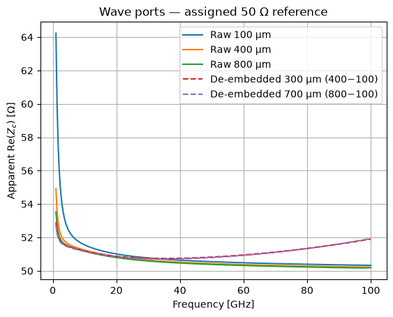
to_skrf(z0=50.0)only assigns 50 Ω to it; this notebook does not measure the mode's circuit impedance or renormalize from it. Assigning twice the reference impedance to the same S-matrix doubles \(Z_c\) without changing the extracted index; \(Z_c\), \(R\), and \(L\) scale with the assigned reference, \(G\) and \(C\) inversely. See Palace's port normalization conventions. - Both: the IEEE P370 split of a non-zero-length 2x-thru (next section) gives an exact propagation constant \(\gamma\) but a biased \(Z_c\). The two halves rebuild the thru exactly, yet they are not half-length lines, so the bias grows with frequency. Section-by-section \(\gamma Z_c\) and \(\gamma/Z_c\) can then give a negative conductance even for a passive line. The physical RLGC therefore comes from \(\gamma\) plus an impedance anchor; see Physical line parameters.
# De-embedding requires all four S-parameters, including the output reflection.
networks = {}
for case, result in results_by_case.items():
    port_names = result.port_names
    assert len(port_names) == 2, "Expected a two-port CPW result."
    expected_pairs = {
        (to_port, from_port) for to_port in port_names for from_port in port_names
    }
    assert set(result.keys()) == expected_pairs, (
        "Run both port excitations before de-embedding."
    )
    networks[case] = result.to_skrf(z0=50.0)
    networks[case].frequency.unit = "GHz"
De-embed the 100 µm reference
Split the 100 µm line into mirrored fixtures using IEEE P370 NZC 2x-thru. Assuming the same end fixtures at every length, removing them from the longer simulations leaves 300 µm (400−100) and 700 µm (800−100) sections. These are inferred networks, not separately simulated lines.
For a uniform, symmetric line, use \(Z_c=\sqrt{B/C}\) with nonnegative real part and unwrap the phase of \(e^{\gamma\ell}=(A+D)/2+B/Z_c\). This keeps the propagation constant continuous when a longer line passes through 180° of electrical length. Reconstructing the original networks checks the fixture orientation.
import matplotlib.pyplot as plt
import numpy as np
from scipy.constants import speed_of_light
from skrf.calibration.deembedding import IEEEP370_SE_NZC_2xThru


def _positive_real_branch(z):
    return np.where(np.real(z) < 0, -z, z)


def extract_modal_parameters(net, length_m):
    """Return Zc, gamma and neff of a uniform symmetric 2-port from its ABCD.

    Branch-free: Zc = sqrt(B/C) on the passive branch determines
    sinh(gamma*l) = B/Zc, hence exp(gamma*l) = cosh + sinh, leaving only the
    2*pi of the complex log to unwrap. No eigenvalue selection is involved, so
    the beta*l = pi eigenvalue collision of a low-loss line never arises.
    """
    a = net.a
    A, B, C, D = a[:, 0, 0], a[:, 0, 1], a[:, 1, 0], a[:, 1, 1]

    zc = _positive_real_branch(np.sqrt(B / C))
    cosh_gl = (A + D) / 2
    sinh_gl = B / zc
    exp_gl = cosh_gl + sinh_gl

    gamma_l = np.log(np.abs(exp_gl)) + 1j * np.unwrap(np.angle(exp_gl))
    gamma = gamma_l / length_m

    neff = np.full(len(net), np.nan)
    nonzero = net.f != 0
    neff[nonzero] = (
        np.imag(gamma[nonzero]) * speed_of_light / (2 * np.pi * net.f[nonzero])
    )

    # Symmetry residual: a uniform symmetric line has A == D.
    symmetry_error = np.max(np.abs(A - D) / np.maximum(np.abs(A), 1e-30))

    return {
        "zc": zc,
        "gamma": gamma,
        "neff": neff,
        "symmetry_error": symmetry_error,
    }


def p370_extract(short_2xthru, long_fix_dut_fix, delta_length_m):
    """Extract the additional line length using a mirrored IEEE P370 split."""
    reference_z0 = float(np.real(np.median(short_2xthru.z0[:, 0])))
    deembedding = IEEEP370_SE_NZC_2xThru(
        dummy_2xthru=short_2xthru,
        z0=reference_z0,
        use_z_instead_ifft=True,
        name="100 um non-zero-length 2xThru",
    )
    dut = deembedding.deembed(long_fix_dut_fix)

    # Explicitly reconstruct both topologies to check fixture orientation.
    reconstructed_short = deembedding.s_side1 ** deembedding.s_side2.flipped()
    reconstructed_long = deembedding.s_side1**dut ** deembedding.s_side2.flipped()
    result = extract_modal_parameters(dut, delta_length_m)
    result.update(
        {
            "dut": dut,
            "deembedding": deembedding,
            "split_error": np.max(np.abs(reconstructed_short.s - short_2xthru.s)),
            "reembed_error": np.max(np.abs(reconstructed_long.s - long_fix_dut_fix.s)),
        }
    )
    return result
raw_parameters = {}
deembedded = {}

for port_type in port_types:
    reference = networks[port_type, 100]
    for length_um in lengths_um:
        raw_parameters[port_type, length_um] = extract_modal_parameters(
            networks[port_type, length_um], length_m=length_um * 1e-6
        )
    for total_length_um in lengths_um[1:]:
        remaining_um = total_length_um - 100
        deembedded[port_type, remaining_um] = p370_extract(
            reference,
            networks[port_type, total_length_um],
            delta_length_m=remaining_um * 1e-6,
        )
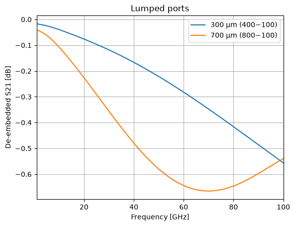
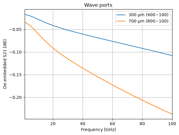
Compare de-embedded transmission
The remaining length still changes the S21 attenuation and phase, even when the sections have the same propagation constant and impedance.
for port_type in port_types:
    plt.figure()
    for remaining_um in (300, 700):
        network = deembedded[port_type, remaining_um]["dut"]
        network.plot_s_db(1, 0, label=f"{remaining_um} µm ({remaining_um + 100}−100)")
    plt.title(port_labels[port_type])
    plt.xlabel("Frequency [GHz]")
    plt.ylabel("De-embedded S21 [dB]")
    plt.grid(True)
    plt.legend()
    plt.show()
Compare index and impedance across lengths
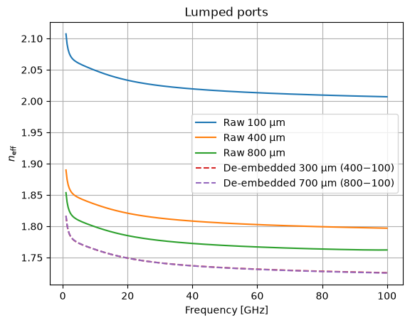
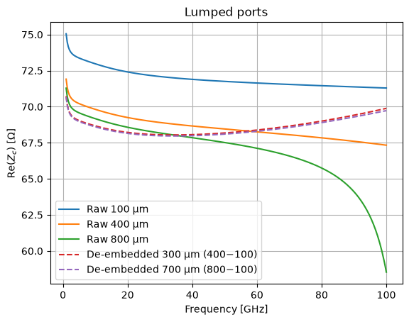
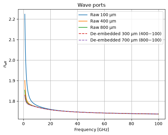
At each frequency, the same uniform line should have the same \(n_{\mathrm{eff}}\) and \(Z_c\) regardless of length. Raw curves include port and end effects; the two de-embedded curves should agree more closely. Both extractions share the same 100 µm reference, so agreement checks consistency rather than independent accuracy or mesh convergence.
Compare the lengths within each port type. The de-embedded \(Z_c\) curves are diagnostic only: wave ports use the assigned 50 Ω reference, and for both port types the P370 split biases \(Z_c\) at high frequency. The physical impedance and RLGC are extracted in the last section from \(\gamma\), which is not affected.
for port_type in port_types:
    for parameter in ("neff", "zc"):
        plt.figure()
        for length_um in lengths_um:
            values = raw_parameters[port_type, length_um][parameter].real
            plt.plot(
                networks[port_type, length_um].f / 1e9,
                values,
                label=f"Raw {length_um} µm",
            )
        for remaining_um in (300, 700):
            parameters = deembedded[port_type, remaining_um]
            plt.plot(
                parameters["dut"].f / 1e9,
                parameters[parameter].real,
                "--",
                label=f"De-embedded {remaining_um} µm ({remaining_um + 100}−100)",
            )
        title = port_labels[port_type]
        if parameter == "neff":
            plt.ylabel(r"$n_{\mathrm{eff}}$")
        elif port_type == "wave":
            plt.ylabel(r"Apparent Re($Z_c$) [Ω]")
            title += " — assigned 50 Ω reference"
        else:
            plt.ylabel(r"Re($Z_c$) [Ω]")
        plt.title(title)
        plt.xlabel("Frequency [GHz]")
        plt.grid(True)
        plt.legend()
        plt.show()
Check the cross-section with a 2D eigensolver
BoundaryModeSim solves directly on the CPW cross-section. At 10, 25, 50, 75, and 100 GHz, compute two guided modes with the wave-port airbox from above, one job per frequency. The solver provides field profiles and complex effective indices. Voltage paths across both gaps also give voltage–power impedance, using Palace's power convention. See Palace's 2D CPW example.
A cross-section carries no 3D port, so add_impedance_path declares the paths directly. They are postprocessing only: they add no 50 Ω termination and excite nothing. Each path runs from the signal to one ground at the conductor's mid-height. The CPW mode should have similar, in-phase voltages across the two gaps; inspect its fields as well as its index. Mode ordering alone does not identify the CPW mode.
This gives an independent check of the index and a physical impedance at a few frequencies; the last section uses it as the impedance anchor of the wave-port fit. The lumped driven model uses a different airbox, so its comparison also includes that difference. Mesh, airbox, and voltage-path convergence still matter. The wave-port curves above retain their assigned 50 Ω reference; the 2D result does not automatically renormalize them.
from gsim.palace import BoundaryModeSim

MODE_FREQUENCIES_GHZ = (10, 25, 50, 75, 100)
mode_job_ids = {}
S_WIDTH, GAP_WIDTH = 20.0, 15.0
metal = get_stack().layers["topmetal2"]
z_mid = 0.5 * (metal.zmin + metal.zmax)

# Same cross-section, mesh settings, and paths at every frequency; only the
# solver frequency (and the output folder name) changes.
for ghz in MODE_FREQUENCIES_GHZ:
    mode_sim = BoundaryModeSim()
    mode_sim.set_output_dir(f"./palace-sim-cpw-2d-wave-{ghz}ghz")
    mode_sim.set_geometry(gsg_electrode())
    mode_sim.set_stack(get_stack())
    mode_sim.set_airbox(margin_x=0, margin_y=50, z_above=100, z_below=100)
    mode_sim.set_cross_section("x=0")
    mode_sim.set_boundary_mode(
        freq=ghz * 1e9, num_modes=2, save=2, target=1.7, tolerance=1e-8
    )
    # A cross-section carries no 3D port. Declare the two signal-to-ground voltage
    # paths directly, in (h, v) = (y, z) microns on the x=0 plane: from the signal
    # conductor edge across the gap to the ground edge, at mid-metal height.
    for sign in (+1.0, -1.0):
        label = "gap 1" if sign > 0 else "gap 2"
        mode_sim.add_impedance_path(
            label,
            voltage=[
                [sign * S_WIDTH / 2, z_mid],
                [sign * (S_WIDTH / 2 + GAP_WIDTH), z_mid],
            ],
            nsamples=200,
        )
    mode_sim.mesh(
        preset="default",
        refined_mesh_size=2,
        max_mesh_size=40,
        fmax=150e9,
        verbose=False,
    )
    mode_job_ids[ghz] = mode_sim.run(wait=False, check_cache=True, verbose="status")
Cache hit: reusing job 01a163e1-cdc1-7367-ae93-47bc3f19f14f


Cache hit: reusing job 01a163e1-d3c7-7115-a1d1-8d0075957d8e


Cache hit: reusing job 01a163e1-d984-7557-b12c-6222df19dec3


Cache hit: reusing job 01a163e1-df77-7507-bb89-bccede943a91


Cache hit: reusing job 01a163e1-7a1a-70e7-978e-d4040c46f0a1
import pandas as pd

from gsim.palace.results import load_text_results

mode_files = gsim.wait_for_results(list(mode_job_ids.values()), verbose="status")
mode_results_by_ghz = {
    ghz: load_text_results(files)
    for ghz, files in zip(mode_job_ids, mode_files, strict=True)
}

mode_tables = {}
cpw_modes = {}
for ghz, results in mode_results_by_ghz.items():
    mode_rows = []
    for mode_number, metrics in results.modes.items():
        voltage_1 = results.mode_voltage(index=1, mode=mode_number)
        voltage_2 = results.mode_voltage(index=2, mode=mode_number)
        impedance_1 = results.characteristic_impedance(index=1, mode=mode_number)
        impedance_2 = results.characteristic_impedance(index=2, mode=mode_number)
        if any(
            value is None for value in (voltage_1, voltage_2, impedance_1, impedance_2)
        ):
            raise ValueError("Missing mode voltage/impedance postprocessing results.")
        voltage_scale = abs(voltage_1) + abs(voltage_2)
        mismatch = (
            abs(voltage_1 - voltage_2) / voltage_scale if voltage_scale else np.inf
        )
        mode_rows.append(
            {
                "Mode": mode_number,
                "Re(n_eff)": metrics["n_eff"].real,
                "Im(n_eff)": metrics["n_eff"].imag,
                "Z_PV gap 1 [Ω]": impedance_1,
                "Z_PV gap 2 [Ω]": impedance_2,
                "Gap-voltage mismatch": mismatch,
            }
        )
    table = pd.DataFrame(mode_rows).set_index("Mode")
    cpw_mode = int(table["Gap-voltage mismatch"].idxmin())
    if table.loc[cpw_mode, "Gap-voltage mismatch"] > 0.1:
        raise ValueError(
            f"No symmetric CPW mode found at {ghz} GHz; inspect the modes."
        )
    mode_tables[ghz] = table
    cpw_modes[ghz] = cpw_mode

# Impedance anchors for the wave-port fit: voltage-power impedance of the CPW
# mode, gap 1. The two gaps must agree.
mode_anchor_frequency_hz = np.array(MODE_FREQUENCIES_GHZ, float) * 1e9
mode_anchor_impedance_ohm = np.array(
    [
        mode_tables[ghz].loc[cpw_modes[ghz], "Z_PV gap 1 [Ω]"]
        for ghz in MODE_FREQUENCIES_GHZ
    ]
)
gap_2_impedance_ohm = np.array(
    [
        mode_tables[ghz].loc[cpw_modes[ghz], "Z_PV gap 2 [Ω]"]
        for ghz in MODE_FREQUENCIES_GHZ
    ]
)
if not np.allclose(gap_2_impedance_ohm, mode_anchor_impedance_ohm, rtol=0.01):
    raise ValueError(
        "Z_PV of the two gaps differs by more than 1 %; inspect the modes."
    )

# The 50 GHz result feeds the comparison and the field plot below.
mode_frequency = 50e9
mode_results = mode_results_by_ghz[50]
mode_table = mode_tables[50]
cpw_mode = cpw_modes[50]
pd.concat(mode_tables, names=["f [GHz]"])
Waiting for 5 jobs...
  palace-020ce1c5                [####################] 100% complete     elapsed 0m 00s
  palace-054b78c9                [####################] 100% complete     elapsed 0m 00s
  palace-b0b34b99                [####################] 100% complete     elapsed 0m 00s
  palace-1a0022e9                [####################] 100% complete     elapsed 0m 00s
  palace-8fbe8f31                [####################] 100% complete     elapsed 0m 00s


Extracting results.tar.gz...
Downloaded 31 files to sim-data-palace-020ce1c5


Extracting results.tar.gz...
Downloaded 31 files to sim-data-palace-054b78c9


Extracting results.tar.gz...
Downloaded 31 files to sim-data-palace-b0b34b99


Extracting results.tar.gz...
Downloaded 31 files to sim-data-palace-1a0022e9


Extracting results.tar.gz...
Downloaded 31 files to sim-data-palace-8fbe8f31
| Re(n_eff) | Im(n_eff) | Z_PV gap 1 [Ω] | Z_PV gap 2 [Ω] | Gap-voltage mismatch | ||
|---|---|---|---|---|---|---|
| f [GHz] | Mode | |||||
| 10 | 1 | 1.768605 | -0.044844 | 70.544624 | 70.779068 | 0.000830 |
| 2 | 1.470419 | -0.020398 | 44.243573 | 43.982371 | 1.000000 | |
| 25 | 1 | 1.752773 | -0.032291 | 70.134110 | 70.361184 | 0.000810 |
| 2 | 1.463155 | -0.014816 | 44.073330 | 43.818149 | 1.000000 | |
| 50 | 1 | 1.742062 | -0.024025 | 69.825698 | 70.043677 | 0.000782 |
| 2 | 1.458405 | -0.011098 | 43.993099 | 43.745422 | 1.000000 | |
| 75 | 1 | 1.737496 | -0.020078 | 69.707284 | 69.919475 | 0.000764 |
| 2 | 1.456644 | -0.009313 | 44.024236 | 43.781297 | 1.000000 | |
| 100 | 1 | 1.734838 | -0.017709 | 69.655480 | 69.863802 | 0.000752 |
| 2 | 1.455911 | -0.008245 | 44.115022 | 43.875194 | 1.000000 |
Compare the CPW mode with the driven extraction
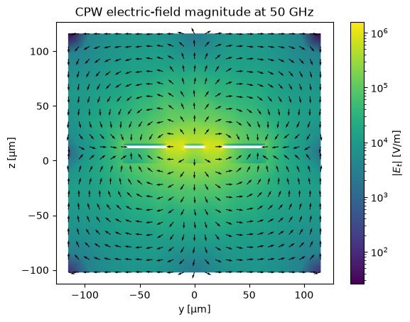
At each frequency, select the mode whose two signal-to-ground voltages agree most closely, and require their relative mismatch to be below 10%. This rejects the opposite gap-voltage signs of a slotline-like mode. Check the field plot below to confirm the mode identity.
Compare at 50 GHz by interpolating the driven sweep. The 2D row uses voltage–power impedance from a specified path. The driven rows show the P370 impedance, which carries the high-frequency bias described above; for wave ports it is also in the assigned 50 Ω reference. So this table checks the effective index, not the impedance. The physical impedance and RLGC come from the fit in the last section.
The heatmap shows transverse electric-field magnitude on a logarithmic color scale. Arrows show direction with phase referenced to the signal-to-ground voltage; their lengths are normalized. Conductor interiors are excluded from the simulation mesh.
cpw_mode = int(mode_table["Gap-voltage mismatch"].idxmin())
if mode_table.loc[cpw_mode, "Gap-voltage mismatch"] > 0.1:
    raise ValueError("No symmetric CPW mode found; inspect the modes.")
comparison_rows = [
    {
        "Model": f"2D CPW mode {cpw_mode}",
        "Airbox": "Wave",
        "Effective index": mode_results.modes[cpw_mode]["n_eff"].real,
        "Impedance [Ω]": mode_results.characteristic_impedance(mode=cpw_mode),
        "Impedance convention": "Voltage–power, gap 1",
    }
]
for port_type in port_types:
    for remaining_um in (300, 700):
        parameters = deembedded[port_type, remaining_um]
        frequency = parameters["dut"].f
        comparison_rows.append(
            {
                "Model": f"{port_labels[port_type]}, de-embedded {remaining_um} µm",
                "Airbox": port_type.capitalize(),
                "Effective index": np.interp(
                    mode_frequency, frequency, parameters["neff"]
                ),
                "Impedance [Ω]": np.interp(
                    mode_frequency, frequency, parameters["zc"].real
                ),
                "Impedance convention": (
                    "Assigned 50 Ω reference"
                    if port_type == "wave"
                    else "Lumped circuit"
                ),
            }
        )
pd.DataFrame(comparison_rows).set_index("Model")
| Airbox | Effective index | Impedance [Ω] | Impedance convention | |
|---|---|---|---|---|
| Model | ||||
| 2D CPW mode 1 | Wave | 1.742062 | 69.825698 | Voltage–power, gap 1 |
| Lumped ports, de-embedded 300 µm | Lumped | 1.736894 | 68.303862 | Lumped circuit |
| Lumped ports, de-embedded 700 µm | Lumped | 1.736702 | 68.226091 | Lumped circuit |
| Wave ports, de-embedded 300 µm | Wave | 1.746740 | 50.905245 | Assigned 50 Ω reference |
| Wave ports, de-embedded 700 µm | Wave | 1.747158 | 50.879711 | Assigned 50 Ω reference |
import pyvista as pv
from matplotlib.colors import LogNorm
from matplotlib.tri import Triangulation

from gsim.palace.results import load_fields

mode_directory = mode_results.files["mode-kn.csv"].parent
field_mesh = (
    load_fields(mode_directory, cycle=cpw_mode)
    .extract_surface(algorithm="dataset_surface")
    .triangulate()
    .clean()
)
# Plot on the native triangles so conductor interiors remain empty.
triangles = field_mesh.faces.reshape(-1, 4)[:, 1:]
triangulation = Triangulation(
    field_mesh.points[:, 0], field_mesh.points[:, 1], triangles
)
electric_field = field_mesh["E_real"] + 1j * field_mesh["E_imag"]
field_magnitude = np.linalg.norm(electric_field, axis=1)

plt.figure()
heatmap = plt.tripcolor(
    triangulation, field_magnitude, shading="gouraud", norm=LogNorm()
)
plt.colorbar(heatmap, label=r"$|E_t|$ [V/m]")
# Sample arrows on a regular grid; exclude points outside the dielectric mesh.
grid_y, grid_z = np.meshgrid(
    np.linspace(field_mesh.bounds[0], field_mesh.bounds[1], 25),
    np.linspace(field_mesh.bounds[2], field_mesh.bounds[3], 20),
)
arrow_points = pv.PolyData(
    np.column_stack((grid_y.ravel(), grid_z.ravel(), np.zeros(grid_y.size)))
).sample(field_mesh)
arrow_field = arrow_points["E_real"] + 1j * arrow_points["E_imag"]
voltage_phase = np.angle(mode_results.mode_voltage(index=1, mode=cpw_mode))
arrow_vectors = np.real(arrow_field * np.exp(-1j * voltage_phase))
arrow_magnitude = np.linalg.norm(arrow_vectors, axis=1)
valid = arrow_points["vtkValidPointMask"].astype(bool) & (arrow_magnitude > 0)
# Arrows show direction only; the heatmap shows magnitude.
arrow_vectors = arrow_vectors[valid] / arrow_magnitude[valid, None]
plt.quiver(
    arrow_points.points[valid, 0],
    arrow_points.points[valid, 1],
    arrow_vectors[:, 0],
    arrow_vectors[:, 1],
    angles="xy",
)
plt.xlabel("y [µm]")
plt.ylabel("z [µm]")
plt.title("CPW electric-field magnitude at 50 GHz")
plt.gca().set_aspect("equal")
plt.grid(False)
plt.show()
Physical line parameters
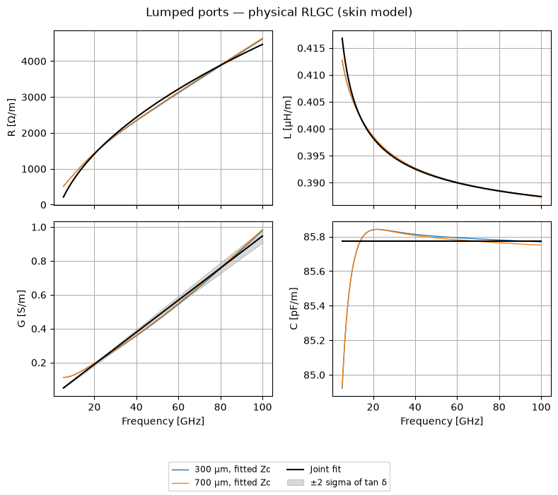
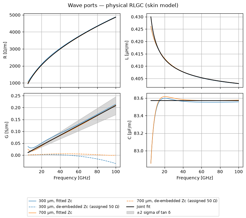
The de-embedded \(\gamma\) is exact, but \(Z_c\) is not: the P370 split biases it, and wave ports only carry an assigned reference. So this section takes only \(\gamma\) from the de-embedded sections and fits one passive line to both sections at once:
A second model without the internal-reactance term \(jR_s\sqrt{f}\) is fitted too, and the one with the lower reduced \(\chi^2\) is used; the wrong model biases \(\tan\delta\). Per-section R, L, G, and C are then \(\gamma Z_c\) and \(\gamma/Z_c\) with the fitted complex \(Z_c=\sqrt{Z/Y}\). Each per-section curve keeps the noise of its own \(\gamma\) (the shorter section is noisier), so small excursions of G around the fit are expected; the joint fit is the physical estimate.
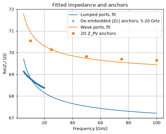
Scale invariance. \(\gamma=\sqrt{ZY}\) does not change under \((R, L, G, C)\to(kR, kL, G/k, C/k)\), so \(\gamma\) cannot fix the impedance level. A few \(Z_c\) magnitudes, the anchors, fix \(k\). A wrong anchor rescales R, L, G, and C together; it cannot flip the sign of G or change \(\tan\delta\).
Anchors.
- Wave ports: the 2D voltage–power impedance at 10, 25, 50, 75, and 100 GHz, from the same airbox as the wave port.
- Lumped ports: the magnitude of the de-embedded \(Z_c\) averaged over 5–20 GHz. The P370 bias is small there (about 1 % for the synthetic lines in the regression test) and, again, only scales R, L, G, and C.
Fit band. Only \(f \ge 5\) GHz is fitted. The simulation models the conductors as a finite-conductivity surface boundary (σ = 3.77e7 S/m, 3 µm thick), and the skin depth at 1 GHz is about 2.6 µm, so a \(\sqrt{f}\) resistance does not hold below a few GHz.
Reading \(\tan\delta\). It is an effective value for this simulation setup, not a material property. The mesh contains SiO₂ (loss tangent 0), SiN (0.001), and air, so dielectric loss alone would give a value between 0 and 1e-3. A larger fitted value means other loss is absorbed into it, for example radiation or leakage into the airbox, port effects, or a conductor loss that does not follow \(\sqrt{f}\). The fit cannot tell these apart, because \(\gamma\) only constrains the total loss.
import numpy as np
from scipy.optimize import least_squares

LINE_MODELS = ("sqrt_f", "skin")


def line_model(params, frequency_hz, model):
    """Return series Z and shunt Y per metre of a passive line.

    Z = R0 + Rs*sqrt(f/1 GHz) [+ j*Rs*sqrt(f/1 GHz)] + j*w*L
    Y = w*C*(tan_delta + j)

    The bracketed term (internal inductance of a skin-effect conductor) is
    included for model "skin" only.
    """
    r0, rs, inductance, capacitance, tan_delta = params
    omega = 2 * np.pi * np.asarray(frequency_hz, float)
    skin = rs * np.sqrt(np.asarray(frequency_hz, float) / 1e9)
    series = r0 + skin + 1j * omega * inductance
    if model == "skin":
        series = series + 1j * skin
    shunt = omega * capacitance * (tan_delta + 1j)
    return series, shunt


def fit_line_parameters(
    frequency_hz,
    sections,
    anchor_frequency_hz,
    anchor_impedance_ohm,
    *,
    gamma_sigma_rel=1e-3,
    impedance_sigma_rel=1e-2,
):
    """Fit one passive line to the gamma of every section plus |Zc| anchors.

    ``sections`` is a list of ``(length_m, gamma)`` pairs on ``frequency_hz``.
    The propagation constant is invariant under
    (R, L, G, C) -> (k*R, k*L, G/k, C/k), so gamma alone cannot fix the
    impedance level. The anchors fix k only: a wrong anchor rescales R, L, G
    and C, but it cannot change the sign of G or the loss tangent.

    Both line models are fitted and the one with the lower reduced chi-square
    is returned as ``best``; ``fits`` holds both, keyed by model name.
    """
    f = np.asarray(frequency_hz, float)
    lengths = np.array([length for length, _ in sections], float)
    gammas = np.array([gamma for _, gamma in sections])
    fa = np.asarray(anchor_frequency_hz, float)
    za = np.asarray(anchor_impedance_ohm, float)
    scale = np.array([100.0, 100.0, 1e-7, 1e-10, 1e-3])
    gamma_sigma = gamma_sigma_rel * np.median(np.abs(gammas))
    # An error dS in a section gives d(gamma) proportional to 1/length.
    weight = lengths / lengths.max()
    beta_per_omega = np.median(gammas.imag / (2 * np.pi * f))
    z_guess = float(np.median(za))
    rs_guess = 2 * z_guess * np.median(gammas.real / np.sqrt(f / 1e9))
    x0 = (
        np.array(
            [0.0, rs_guess, beta_per_omega * z_guess, beta_per_omega / z_guess, 0.0]
        )
        / scale
    )

    fits = {}
    for model in LINE_MODELS:

        def residuals(x, model=model):
            series, shunt = line_model(x * scale, f, model)
            d = (np.sqrt(series * shunt)[None] - gammas) * weight[:, None] / gamma_sigma
            za_series, za_shunt = line_model(x * scale, fa, model)
            dz = (
                np.log(np.abs(np.sqrt(za_series / za_shunt)) / za) / impedance_sigma_rel
            )
            return np.concatenate([d.real.ravel(), d.imag.ravel(), dz])

        # Unbounded on purpose: a negative tan_delta must show up, not be clipped.
        res = least_squares(
            residuals, x0, method="lm", xtol=1e-15, ftol=1e-15, gtol=1e-15
        )
        dof = max(res.fun.size - res.x.size, 1)
        chi2_red = float(res.fun @ res.fun / dof)
        cov = np.linalg.pinv(res.jac.T @ res.jac) * max(chi2_red, 1.0)
        params = res.x * scale
        sigma = np.sqrt(np.clip(np.diag(cov), 0, None)) * scale
        za_series, za_shunt = line_model(params, fa, model)
        names = ("R0", "Rs", "L", "C", "tan_delta")
        fits[model] = {
            "params": dict(zip(names, params, strict=True)),
            "sigma": dict(zip(names, sigma, strict=True)),
            "chi2_red": chi2_red,
            "anchor_error": np.abs(np.sqrt(za_series / za_shunt)) / za - 1,
            "model": model,
        }
    best = min(fits.values(), key=lambda fit: fit["chi2_red"])
    return best, fits


def physical_rlgc(frequency_hz, gamma, fit):
    """Return R, L, G, C of one section from its gamma and the fitted Zc."""
    series, shunt = line_model(list(fit["params"].values()), frequency_hz, fit["model"])
    zc = np.sqrt(series / shunt)
    omega = 2 * np.pi * np.asarray(frequency_hz, float)
    z, y = gamma * zc, gamma / zc
    return {
        "R": z.real,
        "L": z.imag / omega,
        "G": y.real,
        "C": y.imag / omega,
        "zc": zc,
    }
FIT_MIN_GHZ = 5.0
LUMPED_ANCHOR_BAND_GHZ = (5.0, 20.0)
sections_um = (300, 700)

frequency_hz = deembedded["lumped", sections_um[0]]["dut"].f
fit_mask = frequency_hz >= FIT_MIN_GHZ * 1e9
fit_frequency = frequency_hz[fit_mask]

line_fits = {}
anchor_data = {}
for port_type in port_types:
    sections = [
        (um * 1e-6, deembedded[port_type, um]["gamma"][fit_mask]) for um in sections_um
    ]
    if port_type == "wave":
        anchor_frequency = mode_anchor_frequency_hz
        anchor_impedance = mode_anchor_impedance_ohm
    else:
        low, high = (ghz * 1e9 for ghz in LUMPED_ANCHOR_BAND_GHZ)
        band = (fit_frequency >= low) & (fit_frequency <= high)
        anchor_frequency = fit_frequency[band]
        anchor_impedance = np.mean(
            [
                np.abs(deembedded[port_type, um]["zc"][fit_mask][band])
                for um in sections_um
            ],
            axis=0,
        )
    anchor_data[port_type] = (anchor_frequency, anchor_impedance)
    line_fits[port_type] = fit_line_parameters(
        fit_frequency, sections, anchor_frequency, anchor_impedance
    )

fit_rows = []
for port_type, (best, fits) in line_fits.items():
    params, sigma = best["params"], best["sigma"]
    fit_rows.append(
        {
            "Ports": port_labels[port_type],
            "Model": best["model"],
            "χ²_red (skin)": fits["skin"]["chi2_red"],
            "χ²_red (sqrt_f)": fits["sqrt_f"]["chi2_red"],
            "R0 [Ω/m]": params["R0"],
            "Rs [Ω/m at 1 GHz]": params["Rs"],
            "L [µH/m]": params["L"] * 1e6,
            "C [pF/m]": params["C"] * 1e12,
            "tan δ": params["tan_delta"],
            "sigma(tan δ)": sigma["tan_delta"],
            "Max anchor error": np.max(np.abs(best["anchor_error"])),
        }
    )
pd.DataFrame(fit_rows).set_index("Ports")
| Model | χ²_red (skin) | χ²_red (sqrt_f) | R0 [Ω/m] | Rs [Ω/m at 1 GHz] | L [µH/m] | C [pF/m] | tan δ | sigma(tan δ) | Max anchor error | |
|---|---|---|---|---|---|---|---|---|---|---|
| Ports | ||||||||||
| Lumped ports | skin | 0.169925 | 2.967527 | -1060.643708 | 552.716386 | 0.378629 | 85.772338 | 0.017572 | 0.000365 | 0.008314 |
| Wave ports | skin | 0.018289 | 2.160959 | -216.151034 | 507.978037 | 0.394887 | 83.571945 | 0.003965 | 0.000362 | 0.006152 |
units = {"R": "Ω/m", "L": "µH/m", "G": "S/m", "C": "pF/m"}
section_colors = {300: "C0", 700: "C1"}
omega = 2 * np.pi * fit_frequency

for port_type in port_types:
    best, _ = line_fits[port_type]
    series, shunt = line_model(
        list(best["params"].values()), fit_frequency, best["model"]
    )
    fitted = {
        "R": series.real,
        "L": series.imag / omega * 1e6,
        "G": shunt.real,
        "C": shunt.imag / omega * 1e12,
    }
    fig, axes = plt.subplots(2, 2, sharex=True, figsize=(8, 7))
    for um in sections_um:
        parameters = deembedded[port_type, um]
        rlgc = physical_rlgc(fit_frequency, parameters["gamma"][fit_mask], best)
        values = {
            "R": rlgc["R"],
            "L": rlgc["L"] * 1e6,
            "G": rlgc["G"],
            "C": rlgc["C"] * 1e12,
        }
        for axis, parameter in zip(axes.flat, units, strict=True):
            axis.plot(
                fit_frequency / 1e9,
                values[parameter],
                lw=1,
                color=section_colors[um],
                label=f"{um} µm, fitted Zc",
            )
        if port_type == "wave":
            # What the previous reading gave: de-embedded Zc in the assigned reference.
            old_conductance = (parameters["gamma"] / parameters["zc"]).real
            axes[1, 0].plot(
                fit_frequency / 1e9,
                old_conductance[fit_mask],
                "--",
                lw=1,
                color=section_colors[um],
                label=f"{um} µm, de-embedded Zc (assigned 50 Ω)",
            )
    for axis, parameter in zip(axes.flat, units, strict=True):
        axis.plot(fit_frequency / 1e9, fitted[parameter], "k", label="Joint fit")
        axis.set_ylabel(f"{parameter} [{units[parameter]}]")
        axis.grid(True)
    band = 2 * best["sigma"]["tan_delta"] * omega * best["params"]["C"]
    axes[1, 0].fill_between(
        fit_frequency / 1e9,
        fitted["G"] - band,
        fitted["G"] + band,
        color="k",
        alpha=0.15,
        label="±2 sigma of tan δ",
    )
    for axis in axes[1]:
        axis.set_xlabel("Frequency [GHz]")
    # One legend below the panels, so it never covers the data.
    handles, labels = axes[1, 0].get_legend_handles_labels()
    fig.legend(handles, labels, loc="lower center", ncol=2, fontsize="small")
    fig.suptitle(f"{port_labels[port_type]} — physical RLGC ({best['model']} model)")
    fig.tight_layout(rect=(0, 0.04 + 0.035 * ((len(labels) + 1) // 2), 1, 1))
    plt.show()

plt.figure()
for port_type in port_types:
    best, _ = line_fits[port_type]
    series, shunt = line_model(
        list(best["params"].values()), fit_frequency, best["model"]
    )
    (curve,) = plt.plot(
        fit_frequency / 1e9,
        np.sqrt(series / shunt).real,
        label=f"{port_labels[port_type]}, fit",
    )
    anchor_frequency, anchor_impedance = anchor_data[port_type]
    plt.plot(
        anchor_frequency / 1e9,
        anchor_impedance,
        "o" if port_type == "wave" else ".",
        color=curve.get_color(),
        label=(
            "2D Z_PV anchors"
            if port_type == "wave"
            else "De-embedded |Zc| anchors, 5-20 GHz"
        ),
    )
plt.xlabel("Frequency [GHz]")
plt.ylabel(r"Re($Z_c$) [Ω]")
plt.title("Fitted impedance and anchors")
plt.grid(True)
plt.legend()
plt.show()
What each port type gives
| Quantity | Lumped ports | Wave ports |
|---|---|---|
| \(\gamma\), \(n_{\mathrm{eff}}\) from the de-embedded sections | exact | exact |
| \(Z_c\) from the de-embedded sections | biased at high frequency | biased, and in the assigned 50 Ω reference |
| Impedance anchor | de-embedded \(Z_c\) magnitude, 5–20 GHz | 2D voltage–power impedance, 10–100 GHz |
| R, L, G, C | joint fit of \(\gamma\) plus anchor | joint fit of \(\gamma\) plus anchor |
Limits.
- The fit assumes constant L and C, a \(\sqrt{f}\) skin-effect resistance, and a constant loss tangent. CPW dispersion or radiation near 100 GHz would show up as a trend in the anchor residuals and a larger \(\chi^2_{\mathrm{red}}\); in that case, fit only up to the frequency where the residuals stay flat.
- A negative \(R_0\) or a \(\tan\delta\) above what the materials allow means the line model does not describe the simulation completely. Then use the numbers as an effective description of \(\gamma\), not as separate conductor and dielectric losses.
- The anchors set the impedance scale only. An anchor error of a few percent scales R, L, G, and C by that factor and leaves \(\gamma\), \(n_{\mathrm{eff}}\), and \(\tan\delta\) unchanged.
- The lumped and wave airboxes differ, so their fitted L and C need not agree.
- A model-free R, L, G, C per frequency would need a complex, field-based \(Z_c\) for each port type; this notebook does not compute one.