

Differentiable Transmon Circuit Simulation with Circulax#
Required extras
This notebook needs the models and circulax extras:
uv add "qpdk[models,circulax]"
# or, from a checkout of this repository:
uv sync --extra models --extra circulax
# or with pip:
pip install "qpdk[models,circulax]"
See the extras reference for what each extra installs.
This notebook demonstrates how to use Circulax—a differentiable, JAX-based circuit simulator—together with qpdk to design and optimize superconducting transmon qubit circuits.
Circulax formulates circuits as Differential Algebraic Equations (DAEs) and provides automatic differentiation through its solvers, enabling gradient-based inverse design of quantum circuit parameters directly from physical layout dimensions.
Overview#
We showcase two complementary workflows:
Harmonic-Balance (HB) Optimization — Find the periodic steady-state response of a nonlinear transmon circuit under a microwave drive and use
jax.gradto optimize the junction critical current \(I_\text{c}\) and shunt capacitance \(C_\text{s}\) toward target qubit parameters.Transient Pulse Analysis — Simulate the time-domain response of a coupled two-qubit system to a voltage pulse and differentiate a crosstalk metric with respect to the coupling capacitance.
Background#
A transmon qubit is a weakly anharmonic oscillator formed by shunting a Josephson junction (JJ) with a large capacitance [KYG+07, KKY+19].
Following the node-flux formulation of quantum electromagnetic circuits [VD17], the circuit Hamiltonian in the phase basis reads:
where the charging energy \(E_\text{C} = e^2 / (2 C_\Sigma)\) and Josephson energy \(E_\text{J} = \Phi_0 I_\text{c} / (2\pi)\). In the classical circuit picture the junction behaves as a nonlinear inductance:
which Circulax handles naturally through automatic differentiation of the component physics function.
Part 1 — Josephson Junction Harmonic-Balance Optimization#
1.1 Physical Model#
We model a transmon qubit as an LC oscillator with a nonlinear Josephson inductance driven by a weak microwave tone. The goal is to optimize the junction critical current \(I_\text{c}\) and shunt capacitance \(C_\text{s}\) so that the circuit’s transition frequency and anharmonicity match target values.
The Josephson junction’s constitutive relation is:
where \(\varphi = 2\pi\Phi/\Phi_0\) is the dimensionless gauge-invariant phase, with \(\Phi\) the junction flux (integral of voltage). In Circulax, this is implemented as a custom component that returns current contributions (flow equations) and flux storage terms (charge equations).
from circulax.circuit import compile_circuit
from circulax.components.base_component import Signals, States, component
from circulax.components.electronic import Capacitor, Resistor, VoltageSourceAC
1.2 Defining the Josephson Junction Component#
Circulax components are plain Python functions decorated with @component.
They receive port voltages (signals) and internal states (s), and return
two dicts: (f_dict, q_dict) for current and charge contributions.
For the JJ we use a flux-based formulation with an internal state variable
phi representing the junction phase (flux / \(\Phi_0 \cdot 2\pi\)).
FLUX_PER_RAD = Φ_0 / (2.0 * jnp.pi)  # Φ₀/(2π) — flux per unit phase


@component(ports=("p1", "p2"), states=("phi",))
def JosephsonJunction(  # ruff: ignore[invalid-function-name]
    signals: Signals,
    s: States,
    Ic: float = 50e-9,
    R_sub: float = 1e6,
    EJ2_EJ1_ratio: float = 0.0,
) -> tuple[dict, dict]:
    """Josephson junction with multi-harmonic current-phase relation.

    The junction is modelled in the flux formulation:
    - The voltage across the junction equals d(flux)/dt, captured by the
      charge (storage) equation: q['phi'] = -(Φ₀/(2π)) * phi.
    - The supercurrent is I = Ic * [sin(phi) + 2 * (EJ2/EJ1) * sin(2*phi)],
      accounting for higher-order harmonics in inhomogeneous tunnel barriers
      :cite:p:`willschObservationJosephsonHarmonics2024`.
    - A large parallel sub-gap resistance provides DC bias stability.

    Args:
        signals: Port voltages.
        s: Internal states; ``s.phi`` is the gauge-invariant phase.
        Ic: Critical current (1st harmonic) in amperes.
        R_sub: Sub-gap (quasi-particle) resistance in ohms.
        EJ2_EJ1_ratio: Ratio of 2nd to 1st Josephson harmonic energy.
            Typically -0.02 to -0.11 for AlOx junctions.

    Returns:
        Tuple of (flow_dict, charge_dict) for the DAE formulation.
    """
    # Supercurrent with 2nd harmonic correction
    # I(phi) = (2e/hbar) * [EJ1 * sin(phi) + 2 * EJ2 * sin(2*phi)]
    # Ic = (2e/hbar) * EJ1
    i_jj = Ic * (jnp.sin(s.phi) + 2.0 * EJ2_EJ1_ratio * jnp.sin(2.0 * s.phi))

    # Small resistive shunt for numerical stability (sub-gap resistance)
    v_drop = signals.p1 - signals.p2
    i_r = v_drop / R_sub

    # Total current into p1
    i_total = i_jj + i_r

    # Flux-phase relation: V = (Φ₀/2π) * d(phi)/dt
    # In DAE form: f['phi'] = V, q['phi'] = -(Φ₀/2π) * phi
    return (
        {"p1": i_total, "p2": -i_total, "phi": v_drop},
        {"phi": -FLUX_PER_RAD * s.phi},
    )
1.3 Layout-to-Circuit Parameter Mapping#
We map physical dimensions from the qpdk transmon layout to circuit parameters using simple analytical estimates:
Shunt capacitance from the coplanar conformal-mapping formula \(C_\text{s} = \varepsilon_0\, \varepsilon_{\text{eff}}\, L\, K(k')/K(k)\) with \(k = s/(s + 2W)\), where \(s\) is the pad gap, \(W\) the pad width and \(L\) the pad length [CSD+23].
Critical current from the process critical-current density and the JJ area: \(I_\text{c} = J_\text{c} \cdot A_{\text{JJ}}\), with \(J_\text{c} \sim 100\;\text{A/cm}^2\) for Al/AlOx/Al junctions.
from qpdk.models.capacitor import plate_capacitor_capacitance_analytical

# Substrate properties
ε_r_substrate = 11.45  # silicon relative permittivity


def layout_to_circuit_params(
    pad_width_um: float = 250.0,
    pad_height_um: float = 400.0,
    pad_gap_um: float = 15.0,
    jj_area_um2: float = 0.04,
    Jc_A_per_cm2: float = 100.0,
    EJ2_EJ1_ratio: float = 0.0,
) -> dict:
    """Convert layout dimensions to circuit parameters using accurate analytical models.

    Args:
        pad_width_um: Capacitor pad width in μm.
        pad_height_um: Capacitor pad height in μm.
        pad_gap_um: Gap between pads in μm.
        jj_area_um2: Josephson junction area in μm².
        Jc_A_per_cm2: Critical current density in A/cm².
        EJ2_EJ1_ratio: Ratio of 2nd to 1st Josephson harmonic energy. Kept at
            zero here so the circuit matches the sinusoidal analytic targets.

    Returns:
        Dictionary with Cs (shunt capacitance), Ic (critical current), and EJ2_ratio.
    """
    # Shunt capacitance using conformal mapping for coplanar pads
    Cs = plate_capacitor_capacitance_analytical(
        length=pad_height_um,
        width=pad_width_um,
        gap=pad_gap_um,
        ep_r=ε_r_substrate,
    )

    # Critical current from JJ area
    jj_area_cm2 = jj_area_um2 * 1e-8  # μm² to cm²
    Ic = Jc_A_per_cm2 * jj_area_cm2

    return {"Cs": Cs, "Ic": Ic, "EJ2_ratio": EJ2_EJ1_ratio}


# Example: default transmon layout
params = layout_to_circuit_params()
print(f"Shunt capacitance: Cs = {params['Cs'] * 1e15:.2f} fF")
print(f"Critical current:  Ic = {params['Ic'] * 1e9:.2f} nA")

# Derived quantum parameters
E_C = e**2 / (2 * params["Cs"])
E_J = Φ_0 * params["Ic"] / (2 * jnp.pi)
print(f"\nCharging energy:  E_C/h = {E_C / h / 1e9:.3f} GHz")
print(f"Josephson energy: E_J/h = {E_J / h / 1e9:.3f} GHz")
print(f"E_J / E_C = {E_J / E_C:.1f} (transmon regime: >> 1)")
Shunt capacitance: Cs = 69.09 fF
Critical current:  Ic = 40.00 nA

Charging energy:  E_C/h = 0.280 GHz
Josephson energy: E_J/h = 19.867 GHz
E_J / E_C = 70.9 (transmon regime: >> 1)
1.4 Building the Transmon Circuit in Circulax#
We assemble a driven transmon circuit as a netlist: a Josephson junction shunted by a capacitor, with a weak voltage source providing the microwave drive.
# Target qubit parameters
f_target = 5.0e9  # 5 GHz transition frequency
alpha_target = -300e6  # -300 MHz anharmonicity (typical transmon)

# Initial circuit parameters from layout
Cs_init = params["Cs"]
Ic_init = params["Ic"]

# Weak drive parameters
V_drive = 1e-6  # 1 μV drive amplitude (weak probe)
# The classical small-signal resonance of the JJ||Cs circuit is the plasma
# frequency f_p = f01 - alpha, not the transition frequency f01 itself.
f_p_target = f_target - alpha_target  # 5.3 GHz plasma frequency
f_drive = f_p_target


def build_transmon_netlist(Cs: float, Ic: float, EJ2_ratio: float = 0.0) -> dict:
    """Build a driven transmon circuit netlist.

    Args:
        Cs: Shunt capacitance in farads.
        Ic: Junction critical current in amperes.
        EJ2_ratio: Ratio of 2nd to 1st Josephson harmonic energy.

    Returns:
        Circulax-compatible netlist dictionary.
    """
    return {
        "instances": {
            "GND": {"component": "ground"},
            "Vdrive": {
                "component": "source_voltage_ac",
                "settings": {"V": V_drive, "freq": f_drive, "delay": 0.0},
            },
            "Rdrive": {
                "component": "resistor",
                "settings": {"R": 50.0},  # 50 Ω drive impedance
            },
            "JJ1": {
                "component": "josephson_junction",
                "settings": {"Ic": Ic, "R_sub": 1e6, "EJ2_EJ1_ratio": EJ2_ratio},
            },
            "Cs1": {
                "component": "capacitor",
                "settings": {"C": Cs},
            },
        },
        "connections": {
            "GND,p1": ("Vdrive,p2", "JJ1,p2", "Cs1,p2"),
            "Vdrive,p1": "Rdrive,p1",
            "Rdrive,p2": ("JJ1,p1", "Cs1,p1"),
        },
    }


models = {
    "resistor": Resistor,
    "capacitor": Capacitor,
    "josephson_junction": JosephsonJunction,
    # Sinusoidal drive: harmonic balance needs a periodic excitation, so a
    # step source would leave the circuit unexcited (zero AC response).
    "source_voltage_ac": VoltageSourceAC,
    "ground": lambda: 0,
}
1.5 Computing the DC Operating Point#
Before running harmonic balance, we find the DC operating point of the circuit (all time derivatives zero). This serves as the initial guess for the HB solver.
compile_circuit turns the netlist into a callable :class:~circulax.circuit.Circuit.
Compiling once, outside any jax.jit/jax.grad boundary, is what makes the
rest of this notebook differentiable: the circuit topology (and the integer index
arrays derived from it) stays static, while component values are swapped in
functionally through the params= argument of each analysis.
# Compile the netlist into a reusable, differentiable circuit
net_dict = build_transmon_netlist(Cs_init, Ic_init, EJ2_ratio=params["EJ2_ratio"])
circuit = compile_circuit(net_dict, models)
num_vars, port_map = circuit.sys_size, circuit.port_map

# DC operating point
y_dc = circuit.dc()

print(f"System size: {num_vars} state variables")
print(f"DC operating point norm: {jnp.linalg.norm(y_dc):.2e}")
System size: 5 state variables
DC operating point norm: 0.00e+00
1.6 Harmonic-Balance Analysis#
The Harmonic Balance method finds the periodic steady-state of the nonlinear circuit directly in the frequency domain, without stepping through many transient cycles. The state vector \(\mathbf{y}(t)\) is represented by \(K = 2N+1\) equally spaced time samples over one period, and the residual is evaluated in the frequency domain:
# Solve for the periodic steady state at the drive frequency
num_harmonics = 7  # capture up to 7th harmonic for nonlinear response
y_time, y_freq = circuit.hb(freq=f_drive, harmonics=num_harmonics, y0=y_dc)

print(f"HB solution shape: {y_time.shape} (K time samples × {num_vars} vars)")
print(f"Frequency components shape: {y_freq.shape}")

# Extract junction node voltage spectrum
jj_node_idx = port_map["JJ1,p1"]
V_harmonics = jnp.abs(y_freq[:, jj_node_idx])
print("\nJunction node voltage harmonics (first 5):")
for k in range(min(5, len(V_harmonics))):
    print(f"  Harmonic {k}: |V_{k}| = {float(V_harmonics[k]):.4e} V")
HB solution shape: (15, 5) (K time samples × 5 vars)
Frequency components shape: (8, 5)

Junction node voltage harmonics (first 5):
  Harmonic 0: |V_0| = 3.5293e-24 V
  Harmonic 1: |V_1| = 4.9885e-07 V
  Harmonic 2: |V_2| = 2.5763e-23 V
  Harmonic 3: |V_3| = 3.0219e-11 V
  Harmonic 4: |V_4| = 1.2798e-23 V
1.7 Gradient-Based Optimization#
Because Circulax is built entirely in JAX, we can differentiate through the
entire simulation—from physical parameters to output spectra. We define a
loss function that penalizes deviations from the target transition frequency
and use jax.grad + Optax to optimize.
The transition frequency of a transmon is approximately:
where \(E_\text{J} = \Phi_0 I_\text{c}/(2\pi)\) and \(E_\text{C} = e^2/(2C_\Sigma)\).
These closed-form estimates assume a purely sinusoidal current-phase
relation, so the junction’s 2nd harmonic is set to zero for this workflow
(\(E_{\text{J}2}/E_{\text{J}1} = 0\) in layout_to_circuit_params). The component
does support a nonzero ratio \(r\)
[WRW+24], but at leading order such
a term rescales the potential’s quadratic coefficient by \((1+4r)\) and the
anharmonicity by \((1+16r)/(1+4r)\), so the sinusoidal targets above
would no longer describe the circuit.
def transmon_anharmonicity(Ic: ArrayLike, Cs: ArrayLike) -> jax.Array:  # ruff: ignore[unused-function-argument]
    """Compute transmon anharmonicity α ≈ -E_C/h.

    Args:
        Ic: Critical current in amperes (unused, kept for API symmetry).
        Cs: Total shunt capacitance in farads.

    Returns:
        Anharmonicity in Hz (negative).
    """
    E_C_val = e**2 / (2.0 * jnp.asarray(Cs))
    return -E_C_val / h


def transmon_frequency(Ic: ArrayLike, Cs: ArrayLike) -> jax.Array:
    """Compute transmon frequency f01 ≈ (sqrt(8*Ej*Ec) - Ec) / h.

    Args:
        Ic: Critical current in amperes.
        Cs: Total shunt capacitance in farads.

    Returns:
        Transition frequency in Hz.
    """
    E_C_val = e**2 / (2.0 * jnp.asarray(Cs))
    E_J_val = Φ_0 * jnp.asarray(Ic) / (2.0 * jnp.pi)
    return (jnp.sqrt(8.0 * E_J_val * E_C_val) - E_C_val) / h


def hb_loss_fn(params_vec: jax.Array) -> jax.Array:
    """Loss for the HB optimization of Ic and Cs.

    The dominant terms are squared relative errors of the analytic transmon
    f01 and anharmonicity estimates. A weak inverse-response term based on the
    HB 1st harmonic voltage keeps gradients flowing through the simulator.

    Args:
        params_vec: Array [log(Ic), log(Cs)] (log-space for better conditioning).

    Returns:
        Scalar loss value.
    """
    Ic = jnp.exp(params_vec[0])
    Cs = jnp.exp(params_vec[1])

    # Reuse the circuit compiled above and swap in the current parameter values.
    # Recompiling the netlist inside the traced function would turn the
    # topology index arrays into tracers and break the solver setup.
    #
    # The classical circuit resonates at the plasma frequency
    # f_p = f01 - alpha, so the response at the 1st harmonic is maximized when
    # the plasma frequency matches f_p_target. To formulate this as a
    # minimization, we penalize the inverse of the response.
    # For this LC-like circuit with no DC drive, the DC operating point is zero.
    _, y_freq_current = circuit.hb(
        freq=f_p_target,
        harmonics=3,
        y0=jnp.zeros(circuit.sys_size),
        params={"JJ1.Ic": Ic, "Cs1.C": Cs},
    )

    # Extract the 1st harmonic voltage magnitude at the junction node
    jj_node_idx = port_map["JJ1,p1"]
    V_1st_harmonic = jnp.abs(y_freq_current[1, jj_node_idx])

    # Targets: transition frequency and anharmonicity, plus a weak term that
    # keeps the harmonic-balance response in the objective (and therefore keeps
    # the gradient flowing through the simulator).
    f01 = transmon_frequency(Ic, Cs)
    f_error = ((f01 - f_target) / f_target) ** 2

    alpha = transmon_anharmonicity(Ic, Cs)
    alpha_error = ((alpha - alpha_target) / alpha_target) ** 2

    # Inversely proportional to the drive response; epsilon avoids /0
    resonance_loss = 1.0 / (V_1st_harmonic * 1e6 + 1e-12)  # scale V to typical uV range

    return f_error + 0.1 * alpha_error + 0.01 * resonance_loss


# Initial parameters in log-space
params_init = jnp.array([jnp.log(Ic_init), jnp.log(Cs_init)])

# Check initial loss
loss_init = hb_loss_fn(params_init)
print(f"Initial loss: {float(loss_init):.6f}")
Initial loss: 0.098336
1.8 Running the Optimization Loop#
We use Optax (Adam optimizer) to minimize the loss, with jax.grad
providing exact gradients via automatic differentiation.
# Set up the optimizer
optimizer = optax.adam(learning_rate=0.02)
opt_state = optimizer.init(params_init)

params_opt = params_init
losses = []
freq_history = []

# Compile the gradient function
grad_fn = jax.jit(jax.grad(hb_loss_fn))
loss_jit = jax.jit(hb_loss_fn)

# Optimization loop
n_steps = 150
for step in range(n_steps):
    grads = grad_fn(params_opt)
    updates, opt_state = optimizer.update(grads, opt_state)
    params_opt = cast(jax.Array, optax.apply_updates(params_opt, updates))

    loss_val = float(loss_jit(params_opt))
    losses.append(loss_val)

    Ic_cur = float(jnp.exp(params_opt[0]))
    Cs_cur = float(jnp.exp(params_opt[1]))
    f01_cur = float(transmon_frequency(Ic_cur, Cs_cur))
    freq_history.append(f01_cur)

    if step % 50 == 0 or step == n_steps - 1:
        print(f"Step {step:3d}: loss = {loss_val:.2e}, f01 = {f01_cur / 1e9:.4f} GHz")

# Final optimized parameters
Ic_opt = float(jnp.exp(params_opt[0]))
Cs_opt = float(jnp.exp(params_opt[1]))
f01_opt = float(transmon_frequency(Ic_opt, Cs_opt))
alpha_opt = float(transmon_anharmonicity(Ic_opt, Cs_opt))

print(f"\n{'=' * 60}")
print(f"Optimized:  Ic = {Ic_opt * 1e9:.3f} nA,  Cs = {Cs_opt * 1e15:.2f} fF")
print(f"Achieved:   f01 = {f01_opt / 1e9:.4f} GHz,  α = {alpha_opt / 1e6:.1f} MHz")
print(f"Target:     f01 = {f_target / 1e9:.4f} GHz,  α = {alpha_target / 1e6:.1f} MHz")
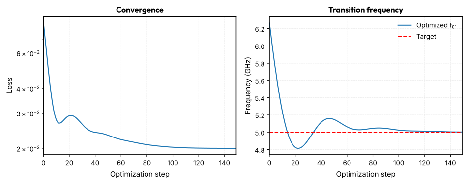
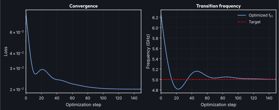
Step   0: loss = 8.51e-02, f01 = 6.2686 GHz
Step  50: loss = 2.32e-02, f01 = 5.1469 GHz
Step 100: loss = 2.03e-02, f01 = 5.0235 GHz
Step 149: loss = 2.00e-02, f01 = 5.0021 GHz

============================================================
Optimized:  Ic = 23.662 nA,  Cs = 64.81 fF
Achieved:   f01 = 5.0021 GHz,  α = -298.9 MHz
Target:     f01 = 5.0000 GHz,  α = -300.0 MHz
1.9 Optimization Convergence#
_, (ax1, ax2) = plt.subplots(1, 2, figsize=(10, 4))

ax1.semilogy(losses)
ax1.set_xlabel("Optimization step")
ax1.set_ylabel("Loss")
ax1.set_title("Convergence")
ax1.grid(True, alpha=0.3)

ax2.plot([f / 1e9 for f in freq_history], label="Optimized $f_{01}$")
ax2.axhline(f_target / 1e9, color="r", linestyle="--", label="Target")
ax2.set_xlabel("Optimization step")
ax2.set_ylabel("Frequency (GHz)")
ax2.set_title("Transition frequency")
ax2.legend()
ax2.grid(True, alpha=0.3)

plt.tight_layout()
plt.show()
1.10 Updated Layout Visualization#
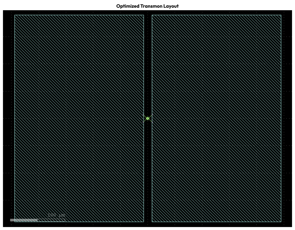
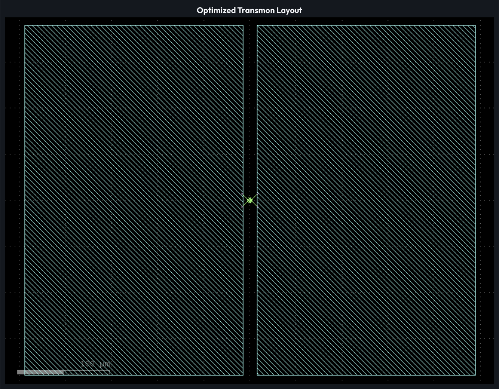
We can now visualize the transmon layout with the optimized dimensions. The inversion below targets the shunt capacitance \(C_\text{s}\) only: the pads are resized so the conformal-mapping model reproduces \(C_\text{s}^{\text{opt}}\), while the junction keeps the default SQUID spec used throughout the PDK. Realizing \(I_\text{c}^{\text{opt}}\) in layout would additionally require sizing the junction overlap area \(A = I_\text{c}^{\text{opt}} / J_\text{c}\) for the process critical-current density, which is a process-level decision outside the scope of this conformal-mapping inversion.
# Compute updated pad dimensions from optimized Cs by inverting the same
# conformal-mapping model used in layout_to_circuit_params. No closed-form
# inverse exists, but the capacitance is monotonic in pad size, so we bisect
# on the pad height with the aspect ratio and gap held fixed.
pad_gap_inv_um = 15.0  # keep gap fixed
aspect = 5.0 / 8.0  # keep aspect ratio ≈ 250:400 = 5:8 (width:height)


def capacitance_for_height(pad_height_um: float) -> jax.Array:
    """Forward-model capacitance of pads with the given height and fixed aspect."""
    return plate_capacitor_capacitance_analytical(
        length=pad_height_um,
        width=aspect * pad_height_um,
        gap=pad_gap_inv_um,
        ep_r=ε_r_substrate,
    )


lo, hi = 1.0, 1e4  # bracketing range in μm
for _ in range(100):
    mid = 0.5 * (lo + hi)
    if capacitance_for_height(mid) < Cs_opt:
        lo = mid
    else:
        hi = mid
pad_height_opt = 0.5 * (lo + hi)
pad_width_opt = aspect * pad_height_opt

# kfactory ports require widths to be even multiples of the 1 nm database unit
pad_height_opt = round(pad_height_opt / 0.002) * 0.002
pad_width_opt = round(pad_width_opt / 0.002) * 0.002

print(f"Optimized pad dimensions: {pad_width_opt:.1f} × {pad_height_opt:.1f} μm²")

# Create the transmon component with optimized dimensions
transmon_opt = double_pad_transmon(
    pad_size=(pad_width_opt, pad_height_opt),
    pad_gap=15.0,
)
transmon_opt.plot()
plt.title("Optimized Transmon Layout")
plt.show()
Optimized pad dimensions: 237.0 × 379.2 μm²
Part 2 — Transient Pulse Analysis and Crosstalk Sensitivity#
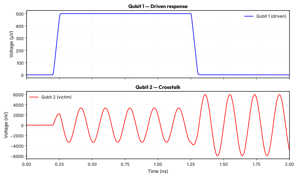
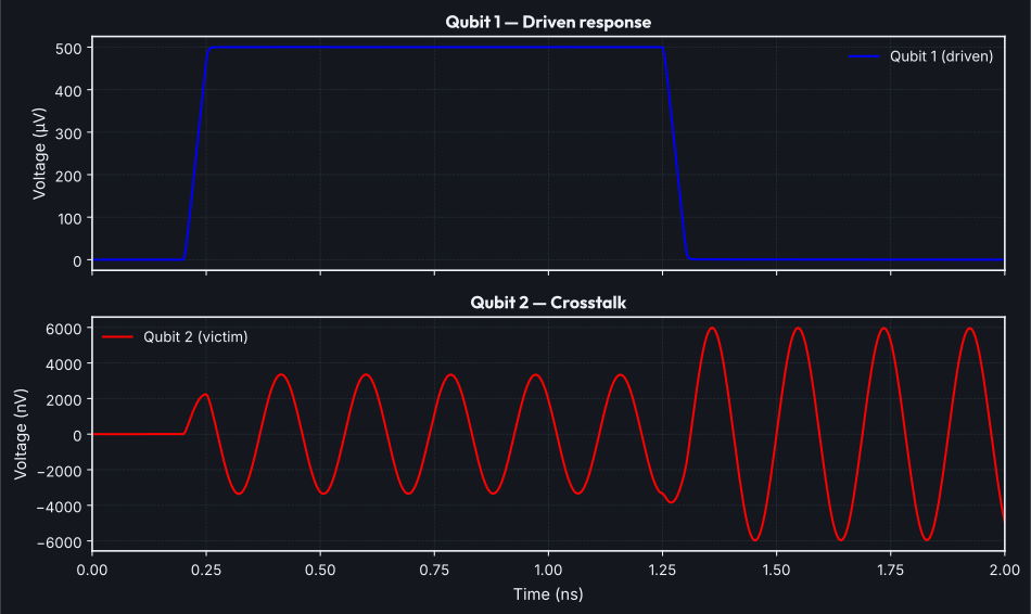
2.1 Coupled Qubit Model#
We model two adjacent transmon qubits coupled through a parasitic mutual capacitance \(C_\text{m}\) [KKY+19, VD17]. A voltage pulse is applied to qubit 1, and we observe the induced response on qubit 2 (crosstalk).
The circuit topology:
@component(ports=("p1", "p2"))
def CouplingCapacitor(  # ruff: ignore[invalid-function-name]
    signals: Signals,
    s: States,  # ruff: ignore[unused-function-argument]
    Cm: float = 1e-15,
) -> tuple[dict, dict]:
    """Mutual coupling capacitor between two nodes.

    Args:
        signals: Port voltages.
        s: Unused; required by the component protocol.
        Cm: Coupling capacitance in farads.

    Returns:
        Tuple of (flow_dict, charge_dict) for the DAE formulation.
    """
    v_drop = signals.p1 - signals.p2
    q_val = Cm * v_drop
    return {}, {"p1": q_val, "p2": -q_val}
2.2 Two-Qubit Coupled Circuit#
We build a netlist with two transmon qubits coupled by a parasitic capacitance. A fast voltage pulse drives qubit 1, and we monitor the voltage at qubit 2’s junction node.
# Circuit parameters for two coupled qubits
Cs_q1 = Cs_opt  # optimized qubit 1
Cs_q2 = Cs_opt  # identical qubit 2
Ic_q1 = Ic_opt
Ic_q2 = Ic_opt * 1.05  # slightly detuned for realism
Cm_init = 0.5e-15  # 0.5 fF coupling capacitance (parasitic)

# Drive pulse parameters
V_pulse = 0.5e-3  # 0.5 mV pulse amplitude
pulse_delay = 0.2e-9  # 200 ps delay
pulse_rise = 50e-12  # 50 ps rise/fall time
pulse_width = 1.0e-9  # 1 ns pulse width
# PulseVoltageSource is periodic; a period far beyond the simulation window
# keeps the drive a single pulse.
pulse_period = 1e-3

coupled_netlist = {
    "instances": {
        "GND": {"component": "ground"},
        # Drive pulse for qubit 1
        "Vpulse": {
            "component": "pulse_source",
            "settings": {
                "v1": 0.0,
                "v2": V_pulse,
                "td": pulse_delay,
                "tr": pulse_rise,
                "tf": pulse_rise,
                "pw": pulse_width,
                "per": pulse_period,
            },
        },
        "Rdrive": {"component": "resistor", "settings": {"R": 50.0}},
        # Qubit 1
        "JJ1": {"component": "josephson_junction", "settings": {"Ic": Ic_q1}},
        "Cs1": {"component": "capacitor", "settings": {"C": Cs_q1}},
        # Qubit 2 (victim)
        "JJ2": {"component": "josephson_junction", "settings": {"Ic": Ic_q2}},
        "Cs2": {"component": "capacitor", "settings": {"C": Cs_q2}},
        # Coupling capacitor (parasitic)
        "Cm": {"component": "coupling_cap", "settings": {"Cm": Cm_init}},
    },
    "connections": {
        "GND,p1": ("Vpulse,p2", "JJ1,p2", "Cs1,p2", "JJ2,p2", "Cs2,p2"),
        "Vpulse,p1": "Rdrive,p1",
        "Rdrive,p2": ("JJ1,p1", "Cs1,p1", "Cm,p1"),
        "Cm,p2": ("JJ2,p1", "Cs2,p1"),
    },
}

# Add the pulse source and coupling cap to models
from circulax.components.electronic import PulseVoltageSource

models_coupled = {
    "resistor": Resistor,
    "capacitor": Capacitor,
    "josephson_junction": JosephsonJunction,
    "coupling_cap": CouplingCapacitor,
    "pulse_source": PulseVoltageSource,
    "ground": lambda: 0,
}

# Compile the coupled circuit once — as in Part 1, the compiled circuit is
# reused for both the nominal run and the differentiable crosstalk metric.
circuit_c = compile_circuit(coupled_netlist, models_coupled, backend="dense")
num_vars_c, port_map_c = circuit_c.sys_size, circuit_c.port_map
y_dc_c = circuit_c.dc()

print(f"Coupled system size: {num_vars_c} variables")
print(f"Port map keys: {list(port_map_c.keys())}")
Coupled system size: 7 variables
Port map keys: ['Cm,p1', 'Cs1,p1', 'JJ1,p1', 'Rdrive,p2', 'Cm,p2', 'Cs2,p1', 'JJ2,p1', 'Cs1,p2', 'Cs2,p2', 'GND,p1', 'JJ1,p2', 'JJ2,p2', 'Vpulse,p2', 'Rdrive,p1', 'Vpulse,p1', 'JJ1,phi', 'JJ2,phi', 'Vpulse,i_src']
2.3 Transient Simulation#
We use Circulax’s transient solver (built on Diffrax) to simulate the time-domain response. For the dense backend the solver steps with the implicit trapezoidal rule at a constant step size, which is stable for stiff circuits.
import diffrax

# Time parameters
t_end = 2.0e-9  # 2 ns simulation
dt0 = 1e-12  # 1 ps initial timestep
n_save = 500  # number of saved points

# Run transient simulation
t_save = jnp.linspace(0, t_end, n_save)
sol = circuit_c.transient(
    t0=0.0,
    t1=t_end,
    dt0=dt0,
    y0=y_dc_c,
    saveat=diffrax.SaveAt(ts=t_save),
    max_steps=200_000,
)

# A failed integration still returns a Solution object, so check the status
# explicitly before trusting the waveform.
if sol.result != diffrax.RESULTS.successful:
    raise RuntimeError(f"Transient solve failed: {sol.result}")

# Extract voltages at qubit nodes
q1_idx = port_map_c["JJ1,p1"]
q2_idx = port_map_c["JJ2,p1"]

v_q1 = sol.ys[:, q1_idx]
v_q2 = sol.ys[:, q2_idx]

print(f"Simulation completed: {n_save} time points")
print(f"Max Q1 voltage: {float(jnp.max(jnp.abs(v_q1))):.4e} V")
print(f"Max Q2 voltage: {float(jnp.max(jnp.abs(v_q2))):.4e} V (crosstalk)")

# Crosstalk ratio
crosstalk_ratio = float(jnp.max(jnp.abs(v_q2))) / (
    float(jnp.max(jnp.abs(v_q1))) + 1e-30
)
print(
    f"Crosstalk ratio: {crosstalk_ratio:.4f} ({20 * jnp.log10(crosstalk_ratio):.1f} dB)"
)
Simulation completed: 500 time points
Max Q1 voltage: 5.0016e-04 V
Max Q2 voltage: 5.9840e-06 V (crosstalk)
Crosstalk ratio: 0.0120 (-38.4 dB)
2.4 Time-Domain Waveforms#
_, (ax1, ax2) = plt.subplots(2, 1, figsize=(10, 6), sharex=True)

t_ns = t_save * 1e9

ax1.plot(t_ns, v_q1 * 1e6, "b-", linewidth=1.5, label="Qubit 1 (driven)")
ax1.set_ylabel("Voltage (μV)")
ax1.set_title("Qubit 1 — Driven response")
ax1.legend()
ax1.grid(True, alpha=0.3)

ax2.plot(t_ns, v_q2 * 1e9, "r-", linewidth=1.5, label="Qubit 2 (victim)")
ax2.set_xlabel("Time (ns)")
ax2.set_ylabel("Voltage (nV)")
ax2.set_title("Qubit 2 — Crosstalk")
ax2.legend()
ax2.grid(True, alpha=0.3)

plt.tight_layout()
plt.show()
2.5 Crosstalk Sensitivity Analysis#
We use jax.grad to differentiate the peak crosstalk voltage with respect
to \(\log C_\text{m}\). The resulting sensitivity
\(\partial V_{\text{peak}}/\partial \log C_m = C_m \, \partial
V_{\text{peak}}/\partial C_m\) has units of volts: it is the absolute
change in peak victim voltage per unit fractional change in \(C_\text{m}\),
which in a real design is set by the physical spacing between qubits.
Since Circulax runs entirely in JAX, the gradient flows through the ODE solver back to the circuit parameters, so the same machinery could drive end-to-end optimization of layout parameters against time-domain metrics.
def crosstalk_metric(log_Cm: ArrayLike) -> jax.Array:
    """Compute peak crosstalk voltage as a function of coupling capacitance.

    This function is differentiable w.r.t. log_Cm via JAX autodiff.

    Args:
        log_Cm: Natural log of coupling capacitance.

    Returns:
        Peak absolute voltage at qubit 2 (the victim).
    """
    Cm_val = jnp.exp(log_Cm)

    # Reuse the compiled circuit and update only the coupling capacitance.
    # The gradient flows through the ODE solve into `Cm`.
    sol_val = circuit_c.transient(
        t0=0.0,
        t1=t_end,
        dt0=dt0,
        saveat=diffrax.SaveAt(ts=t_save),
        max_steps=200_000,
        params={"Cm.Cm": Cm_val},
    )

    # Get Q2 voltage
    v_victim = sol_val.ys[:, q2_idx]
    return jnp.max(jnp.abs(v_victim))


# Absolute voltage sensitivity per fractional change in Cm:
# dV_peak/dlog(Cm) = Cm * dV_peak/dCm
log_Cm = jnp.log(Cm_init)
grad_crosstalk = jax.grad(crosstalk_metric)(log_Cm)

print(f"Coupling capacitance: Cm = {Cm_init * 1e15:.3f} fF")
print(f"∂(crosstalk)/∂(log Cm) = {float(grad_crosstalk):.4e}")
if grad_crosstalk > 0:
    print("\nCrosstalk grows with Cm, so reducing Cm (increasing")
    print("qubit-qubit spacing in the layout) reduces crosstalk.")
else:
    print("\nCrosstalk does not grow with Cm at this operating point.")
Coupling capacitance: Cm = 0.500 fF
∂(crosstalk)/∂(log Cm) = 6.7849e-06

Crosstalk grows with Cm, so reducing Cm (increasing
qubit-qubit spacing in the layout) reduces crosstalk.
Summary#
This notebook demonstrated two key capabilities enabled by Circulax’s differentiable circuit simulation framework:
Harmonic-Balance Optimization — We defined a nonlinear Josephson junction component, assembled a driven transmon circuit, and used
jax.gradto optimize the junction parameters toward a target qubit frequency.Transient Crosstalk Analysis — We simulated a pulse driving one qubit in a coupled two-qubit system and computed gradients of the crosstalk voltage with respect to the coupling capacitance, quantifying how sensitive the parasitic coupling is to layout choices.
Key Takeaways#
Circulax makes it straightforward to define custom nonlinear components (like Josephson junctions) as plain Python functions.
The entire simulation stack is differentiable, enabling gradient-based optimization of physical parameters.
The JAX ecosystem (Optax, Diffrax, Optimistix) provides a unified framework for simulation, optimization, and analysis.
Physical layout parameters from qpdk map directly to circuit parameters, closing the loop between design and simulation.
References#
Qi-Ming Chen, Priyank Singh, Rostislav Duda, Giacomo Catto, Aarne Keränen, Arman Alizadeh, Timm Mörstedt, Aashish Sah, András Gunyhó, Wei Liu, and Mikko Möttönen. Compact inductor-capacitor resonators at sub-gigahertz frequencies. Physical Review Research, 5(4):043126, November 2023. doi:10.1103/PhysRevResearch.5.043126.
Jens Koch, Terri M. Yu, Jay Gambetta, A. A. Houck, D. I. Schuster, J. Majer, Alexandre Blais, M. H. Devoret, S. M. Girvin, and R. J. Schoelkopf. Charge-insensitive qubit design derived from the Cooper pair box. Physical Review A, 76(4):042319, October 2007. doi:10.1103/PhysRevA.76.042319.
P. Krantz, M. Kjaergaard, F. Yan, T. P. Orlando, S. Gustavsson, and W. D. Oliver. A quantum engineer's guide to superconducting qubits. Applied Physics Reviews, 6(2):021318, June 2019. doi:10.1063/1.5089550.
Uri Vool and Michel Devoret. Introduction to quantum electromagnetic circuits. International Journal of Circuit Theory and Applications, 45(7):897–934, July 2017. doi:10.1002/cta.2359.
Dennis Willsch, Dennis Rieger, Patrick Winkel, Madita Willsch, Christian Dickel, Jonas Krause, Yoichi Ando, Raphaël Lescanne, Zaki Leghtas, Nicholas T. Bronn, Pratiti Deb, Olivia Lanes, Zlatko K. Minev, Benedikt Dennig, Simon Geisert, Simon Günzler, Sören Ihssen, Patrick Paluch, Thomas Reisinger, Roudy Hanna, Jin Hee Bae, Peter Schüffelgen, Detlev Grützmacher, Luiza Buimaga-Iarinca, Cristian Morari, Wolfgang Wernsdorfer, David P. DiVincenzo, Kristel Michielsen, Gianluigi Catelani, and Ioan M. Pop. Observation of josephson harmonics in tunnel junctions. Nature Physics, 20(5):815–821, May 2024. doi:10.1038/s41567-024-02400-8.
Circulax documentation: https://gdsfactory.github.io/circulax/