Sattari Suspended Silicon Coupler with GDSFactory FDTD
Model a compact silicon coupler suspended in air and calculate its cross and through transmission.
You will: build the component, configure the physical stack and 40 nm grid, preview the domain, and inspect transmission and a field monitor.
Requirements: GDSFactory+ cloud simulation access.
Reference run: 40 nm cells · 49,267,680 total allocated cells, including PML and padding.
Original paper
H. Sattari et al., “Compact broadband suspended silicon photonic directional coupler,” Optics Letters 45, 2997–3000 (2020). Read the paper · DOI 10.1364/OL.394470.
1. Build the component
All geometry below is in micrometers. The model includes fixed 200 nm straight leads at its modal ports.
import math

import gdsfactory as gf
import matplotlib.pyplot as plt
import numpy as np
from gdsfactory.technology import LayerLevel, LayerStack, LogicalLayer

from gsim import fdtd

gf.gpdk.PDK.activate()


def level(layer, material, zmin, thickness):
    return LayerLevel(
        layer=LogicalLayer(layer=layer),
        material=material,
        zmin=zmin,
        thickness=thickness,
        mesh_order=1,
        sidewall_angle=0,
    )
def extend_ports(component, length_um):
    """Append straight access guides and move each existing optical port."""
    ports = list(component.ports)
    component.ports.clear()
    for port in ports:
        angle = math.radians(port.orientation)
        normal = np.round([math.cos(angle), math.sin(angle)], 12)
        tangent = np.array([-normal[1], normal[0]])
        start = np.asarray(port.center)
        # GDS polygons are quantized to 1 nm; ports must share that face.
        end = np.round(start + length_um * normal, 3)
        half_width = port.width / 2
        component.add_polygon(
            [
                start - half_width * tangent,
                end - half_width * tangent,
                end + half_width * tangent,
                start + half_width * tangent,
            ],
            layer=port.layer,
        )
        component.add_port(
            name=port.name,
            center=tuple(end),
            width=port.width,
            orientation=port.orientation,
            layer=port.layer,
        )
component = gf.Component()
# The facing edges remain at±75nm as each arm tapers on its outer edge.
x = np.array([-10.5, -0.5, 0.5, 10.5])
width_um = np.array([0.45, 0.30, 0.30, 0.45])
for sign in (-1, 1):
    inner = sign * np.full_like(x, 0.075)
    outer = sign * (0.075 + width_um)
    component.add_polygon(
        np.column_stack([np.r_[x, x[::-1]], np.r_[inner, outer[::-1]]]), layer=(1, 0)
    )
# Build the quarter-circle strips directly from their inner/outer radii.
angles = np.linspace(-np.pi / 2, 0, 361)
outer = np.column_stack([10.5 + 5.225 * np.cos(angles), 5.3 + 5.225 * np.sin(angles)])
inner = np.column_stack([10.5 + 4.775 * np.cos(angles), 5.3 + 4.775 * np.sin(angles)])
for side_x in (-1, 1):
    for side_y, orientation in [(-1, 270), (1, 90)]:
        polygon = np.vstack([outer, inner[::-1]]) * np.array([side_x, side_y])
        component.add_polygon(polygon, layer=(1, 0))
        name = {(-1, -1): "o1", (-1, 1): "o2", (1, 1): "o3", (1, -1): "o4"}[
            (side_x, side_y)
        ]
        component.add_port(
            name=name,
            center=(side_x * 15.5, side_y * 5.3),
            width=0.45,
            orientation=orientation,
            layer=(1, 0),
        )
layers = {"core": level((1, 0), "Si", 0, 0.214)}

extend_ports(component, 0.2)
2. Configure the simulation
Use explicit layer thicknesses and frozen source-center indices to reproduce the saved result. The 1.28 µm target PML is rounded up to whole cells. Materials are nondispersive over the sweep.
pdk = gf.Pdk(
    name="fdtd_sattari_suspended_coupler", layer_stack=LayerStack(layers=layers)
)
simulation = fdtd.Simulation(pdk=pdk)
simulation.geometry(component)
simulation.materials(background="Air", overrides={"Si": 3.477723756220899, "Air": 1.0})
simulation.source(port="o1", wavelength_um=1.55, wavelength_span_um=0.1)
simulation.solver(cell_size_nm=40, max_wall_seconds=1800)
simulation.domain(
    pml_cells=32,
    x_bounds=((-16.725), (16.725)),
    y_bounds=((-5.5), (5.5)),
    z_bounds=((-1.0), (1.214)),
)

lower, upper = np.array([[-16.725, -5.5, -1.0], [16.725, 5.5, 1.214]])
simulation.monitors.add_plane(
    "overview_xy",
    center_um=((lower[0] + upper[0]) / 2, (lower[1] + upper[1]) / 2, 0.107),
    size_um=(upper[0] - lower[0] - 0.24, upper[1] - lower[1] - 0.24, 0),
    normal="+z",
    flux=False,
    wavelengths_um=[1.55],
    heatmap=fdtd.Heatmap(quantity="intensity", wavelengths_um=[1.55]),
)
PlaneMonitor(name='overview_xy', center_um=(0.0, 0.0, 0.107), size_um=(33.21, 10.76, 0.0), normal='+z', flux=False, wavelengths_um=[1.55], heatmap=Heatmap(quantity='intensity', wavelengths_um=[1.55]), fiber_mode=None, fields=None)
3. Inspect the simulation
Use the built-in 2D views to inspect the core, ports, monitor and PML. The top view passes through the core; the side view shows the vertical stack.
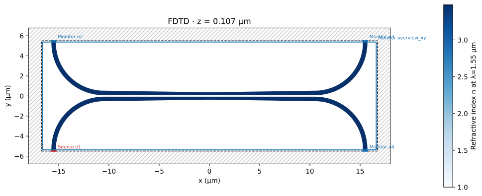
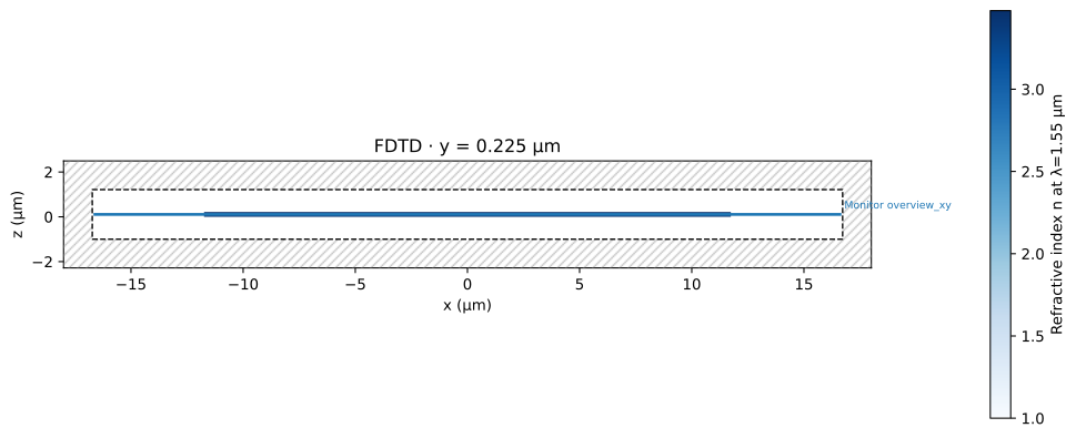
Rotate and zoom the built-in 3D viewer to inspect the complete simulation geometry.
4. Run the simulation
Reuse a matching result when it is available in the cloud cache.
print(f"Total allocated cells: {result.grid['total_cells']:,}")
print(f"Solver time: {result.timing['run_seconds']:.1f} s")
Total allocated cells: 49,267,680
Solver time: 138.4 s
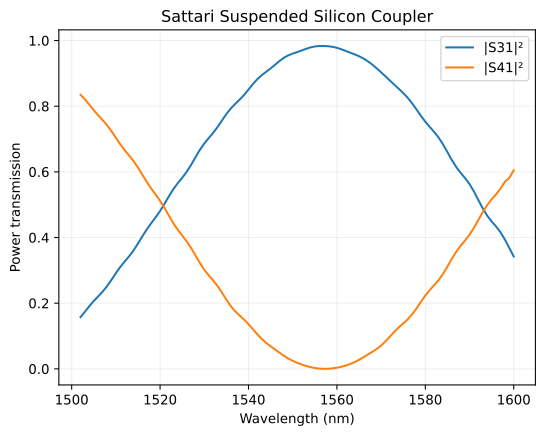
5. Inspect transmission
Plot incident-power-normalized modal transmission. Invalid source-band samples remain masked. Default Matplotlib figure size and fonts are used.
fig, ax = plt.subplots()
for port in ["o3", "o4"]:
    trace = result.s_parameters[port, "o1"]
    power = np.where(trace.valid, np.abs(trace.values) ** 2, np.nan)
    ax.plot(result.wavelength_um * 1000, power, label=f"|S{port[1:]}1|²")
ax.set(
    xlabel="Wavelength (nm)",
    ylabel="Power transmission",
    title="Sattari Suspended Silicon Coupler",
)
ax.grid(alpha=0.2)
ax.legend()
plt.show()
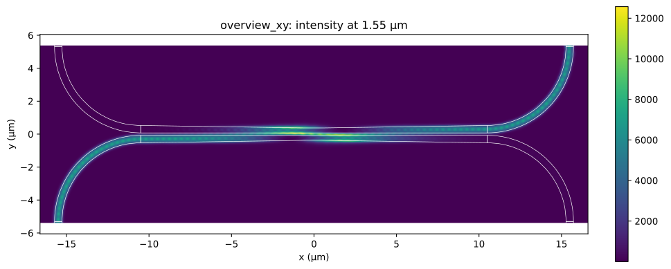
6. Inspect the top-view field
Overlay the silicon or silicon-nitride layout on the source-center intensity monitor. The x/y axes use equal aspect.
monitor = result.monitors["overview_xy"]
fig, ax = plt.subplots(figsize=(10, 4), layout="constrained")
monitor.plot_heatmap(
    wavelength_um=simulation.source.wavelength_um,
    quantity="intensity",
    ax=ax,
    cmap="viridis",
)
for points in component.get_polygons_points(by="tuple")[(1, 0)]:
    outline = np.vstack([points, points[0]])
    ax.plot(outline[:, 0], outline[:, 1], color="white", linewidth=0.5)
ax.set_aspect("equal", adjustable="box")
plt.show()
Model scope
The nominal optical core has 214 nm silicon, a 300 nm minimum arm width and 150 nm gap. Mechanical anchors, release transitions, roughness and fabricated contour changes are omitted. Compare the paper’s Fig. 6 with that reconstruction in mind; 40 nm is the selected example grid rather than a convergence guarantee.
The saved result reached its finite-time stopping condition. That is separate from spatial mesh convergence. The reference campaign enforced a 30-minute wall-time budget.