TCAD: capacitance of a reverse-biased PN junction¶

How does the small-signal capacitance of a lateral silicon PN junction fall with reverse bias, and how close is it to the textbook depletion approximation?

gsim.tcad solves Poisson and electron/hole drift-diffusion with DEVSIM on a 2D cross-section of the device, on the same mesh the Palace mode solver sees. Each bias point returns the carrier concentrations \(n(x, z)\) and \(p(x, z)\), the terminal currents and the small-signal capacitance \(C = |\mathrm{Im}\,I| / \omega\) from a quasi-static AC solve.

Assumptions. Abrupt, uniformly doped junction; 300 K silicon with Masetti mobility; ohmic contacts; Poisson solved in the doped silicon only (the oxide around it is a zero-normal-field wall). The 2D device is 1 cm deep, so extensive quantities come back per cm of device length (*_per_cm), with *_per_m conversions alongside.

Units. Lengths in µm, concentrations in cm⁻³, voltages in V, frequencies in Hz. Field names carry their unit.

Requirements: the tcad extra, pip install "gsim[tcad]".

The device¶

A 220 nm silicon rib cut into four doped strips along \(y\): an n contact pad, the n half of the junction, the p half and a p contact pad, with an aluminium electrode on each pad. The pads keep the ohmic contacts away from the metallurgical junction, so their equilibrium boundary condition does not distort the depletion region.

import gdsfactory as gf

from gsim.common.cross_section import build_doped_cross_section
from gsim.common.stack.extractor import Layer
from gsim.common.stack.materials import make_doped_materials

gf.gpdk.PDK.activate()

CENTER_Y = -20.0  # junction position (um)
FLANK = 0.3  # width of each junction half (um)
PAD = 0.5  # width of each contact pad (um)
RIB_HEIGHT = 0.22  # um
N_A = N_D = 1e18  # cm^-3

spans = {
    "n_pad": (CENTER_Y - FLANK - PAD, CENTER_Y - FLANK),
    "n_rib": (CENTER_Y - FLANK, CENTER_Y),
    "p_rib": (CENTER_Y, CENTER_Y + FLANK),
    "p_pad": (CENTER_Y + FLANK, CENTER_Y + FLANK + PAD),
}
electrodes = {"n_pad": "cathode_metal", "p_pad": "anode_metal"}

component = gf.Component()
component << gf.c.rectangle((10.0, 100.0), centered=True, layer=(3, 0))
layers = {}
for i, (name, (y0, y1)) in enumerate(spans.items()):
    strip = component << gf.c.rectangle((10.0, y1 - y0), layer=(30, i))
    strip.y = (y0 + y1) / 2
    layers[name] = Layer(
        name=name,
        gds_layer=(30, i),
        zmin=0.0,
        zmax=RIB_HEIGHT,
        thickness=RIB_HEIGHT,
        material=name,
        layer_type="dielectric",
        mesh_resolution="fine",
    )
for i, (pad, electrode) in enumerate(electrodes.items()):
    y0, y1 = spans[pad]
    metal = component << gf.c.rectangle((10.0, y1 - y0), layer=(46, i))
    metal.y = (y0 + y1) / 2
    layers[electrode] = Layer(
        name=electrode,
        gds_layer=(46, i),
        zmin=RIB_HEIGHT,
        zmax=RIB_HEIGHT + 0.5,
        thickness=0.5,
        material="aluminum",
        layer_type="conductor",
        mesh_resolution="fine",
    )

stack, _ = build_doped_cross_section(
    component,
    axis="x",
    value=0.0,
    substrate_thickness=2.0,
    doping={
        "layer_specs": layers,
        "materials": make_doped_materials(
            [(n, 1.6e3) for n in spans], permittivity=11.9
        ),
    },
    verbose=False,
)

Configure the simulation¶

The simulation is set up by physical concern: the geometry and its stack, the cross-section domain, the doping, the contacts and interfaces, and the solver. A Contact is where an electrode meets a doped Region; an Interface is where two doped Regions meet, with potential and carriers continuous across it.

from gsim import tcad

sim = tcad.Simulation()
sim.geometry(component, stack=stack)
sim.domain(
    plane="x=0",
    window=(CENTER_Y - 1.2, CENTER_Y + 1.2),
    margin_y=0.5,
    z_above=1.0,
    z_below=1.0,
)

for region in ("n_pad", "n_rib"):
    sim.doping.add(
        tcad.StepDoping(region=region, dopant_type="donor", concentration_cm3=N_D)
    )
for region in ("p_rib", "p_pad"):
    sim.doping.add(
        tcad.StepDoping(region=region, dopant_type="acceptor", concentration_cm3=N_A)
    )

sim.contacts.add(name="cathode", semiconductor="n_pad", electrode="cathode_metal")
sim.contacts.add(name="anode", semiconductor="p_pad", electrode="anode_metal")
sim.interfaces.add(name="n_link", region_a="n_pad", region_b="n_rib")
sim.interfaces.add(name="junction", region_a="n_rib", region_b="p_rib")
sim.interfaces.add(name="p_link", region_a="p_rib", region_b="p_pad")

# The depletion edges move with bias: hold the mesh fine over the strip they sweep.
sim.solver(
    mesh_preset="coarse",
    refined_mesh_size_um=0.02,
    max_mesh_size_um=40.0,
    refinement_boxes=[(CENTER_Y - 0.12, CENTER_Y + 0.12, 0.0, RIB_HEIGHT, 0.01)],
)
mesh = sim.mesh(output_dir="./tcad-sim-pn-junction")

Sweep the reverse bias¶

Raising the cathode (n side) above the anode reverse-biases the junction. Between bias points the contact is ramped in solver.bias_step_v steps so each Newton solve starts close to its answer.

import numpy as np

biases = np.linspace(0.0, 2.0, 5)
sweep = sim.sweep(biases, contact="cathode")

Carriers across the junction¶

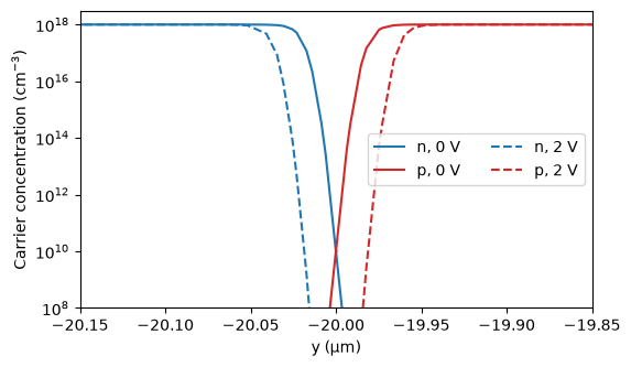
A cut across the rib at mid height shows the depletion region: the strip around the junction at \(y = -20\) µm emptied of mobile carriers, which widens with reverse bias.

import matplotlib.pyplot as plt

fig, ax = plt.subplots(figsize=(6, 3.5))
for point, style in ((sweep.points[0], "-"), (sweep.points[-1], "--")):
    c = point.carriers
    cut = np.abs(c.y_um - RIB_HEIGHT / 2) < 0.01
    order = np.argsort(c.x_um[cut])
    y = c.x_um[cut][order]
    ax.semilogy(
        y, c.electrons_cm3[cut][order], "C0" + style, label=f"n, {point.bias_v:.0f} V"
    )
    ax.semilogy(
        y, c.holes_cm3[cut][order], "C3" + style, label=f"p, {point.bias_v:.0f} V"
    )
ax.set_xlim(CENTER_Y - 0.15, CENTER_Y + 0.15)
ax.set_ylim(1e8, 3e18)
ax.set_xlabel("y (µm)")
ax.set_ylabel("Carrier concentration (cm$^{-3}$)")
ax.legend(ncol=2, loc="center right")
plt.show()

png

C(V) against the depletion approximation¶

For an abrupt junction the depletion approximation (Sze, Physics of Semiconductor Devices, ch. 2) gives \(C_j = \varepsilon_s / W\) per unit area, with \(W \propto \sqrt{V_{bi} + V_R}\). tcad.compare_capacitance evaluates it over the junction face, the rib height times the 1 cm depth, at the same biases, with the solve's own silicon constants (relative permittivity 11.1 and DEVSIM's intrinsic density).

from gsim.common.stack.pn_junction import PNJunctionConfig

comparison = tcad.compare_capacitance(
    PNJunctionConfig(na_cm3=N_A, nd_cm3=N_D), sweep, height_um=RIB_HEIGHT
)

fig, ax = plt.subplots(figsize=(5, 3.5))
ax.plot(
    comparison.v_reverse,
    comparison.c_tcad_f_per_cm * 1e12,
    "o-",
    label="DEVSIM drift-diffusion",
)
ax.plot(
    comparison.v_reverse,
    comparison.c_analytic_f_per_cm * 1e12,
    "--",
    label="Depletion approximation",
)
ax.set_xlabel("Reverse bias $V_R$ (V)")
ax.set_ylabel("Capacitance (pF/cm)")
ax.legend()
plt.show()

print(
    f"largest deviation from the depletion approximation: {comparison.max_relative_deviation:.1%}"
)

png

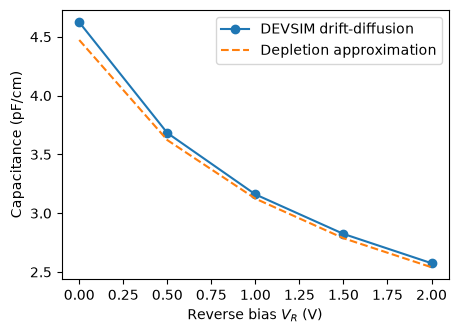
largest deviation from the depletion approximation: 3.4%

Can the result be trusted?¶

Mesh. The depletion edges move with bias, so the elements around the junction must stay well below the depletion width (about 50 nm here at 0 V); the refinement box holds them at 10 nm. Without it the elements there are several times larger and C(V) comes out about 25 % high with a kink where an edge crosses an element. Halve the box size and check that C(V) does not move.
Analytic limit. The two curves should agree to a few percent and have the same slope. What remains is what the depletion approximation leaves out: the mobile-carrier tails at the depletion edges and the field at the rib corners.
Leakage. The reverse current, sweep.points[-1].currents_a_per_cm, should be tiny and balance between the two contacts.

Limits¶

The oxide is left out of the electrostatics, so field lines are forced through the silicon. Declare it with sim.materials(insulators={"sio2": 3.9}) to include the fringing through it.
Every mesh input (geometry, domain, contacts, interfaces, mesh settings) is recorded by mesh(); change one and the next solve asks for mesh() again. A change to the materials, the doping or the solver tolerances rebuilds the DEVSIM device on the existing mesh.
DEVSIM is a process-wide solver: one charge-transport device is live at a time.

Next¶

TCAD guide: the concerns, units, Contacts and Interfaces, and the stale-state rules.
BiasPoint.junction_branch() fits the series resistance and junction capacitance a loaded-line RF model needs.