Differential interconnects, crosstalk, and time-domain reflectometry with Palace
This tutorial addresses gsim #274. We model two IHP SG13G2 signal traces over a common return plane, then cut an asymmetric slot in that plane. Does the slot increase reflections, couple energy between the signals, or convert differential excitation into common mode? Can we locate it from the reflected waveform?
Palace performs the electromagnetic (EM) frequency-domain solve. Python and
scikit-rf perform network conversion and time-domain reflectometry (TDR): the
reflected response to an incident voltage step. The reusable analysis helpers
live in gsim.palace.signal_integrity; this notebook shows how to use them on
a device and how to interpret the result.
The process design kit (PDK) supplies process layers. Geometry helpers accept layer selections, simulation helpers accept a resolved stack, and analysis helpers accept networks and port names. Only the IHP setup section knows IHP layer names. A small synthetic PDK check demonstrates this separation.
Execution: run the notebook in order. The default EXECUTION = "recorded" replays the completed local experiments if
the accompanying run directories are present. The repository strips cell outputs; the numerical discussion below and exported
figures in docs/assets/plots/palace-si-*.png retain selected results. Raw run
archives are not bundled; use local/cloud execution to regenerate them. "preview" runs analytic checks and builds layouts without
meshing or submitting jobs.
Choose "local" or "cloud" to generate EM data, or "load" to analyze the exact
saved experiment. The convergence study is separately enabled. Missing runs are
reported as incomplete, never replaced by analytic curves.
This notebook requires gsim's PDK-authoritative stack API (PR #360; base commit
33fa363b7499a68c2818f72289395739fd76ce55). No helper scripts or measurement files
are required. Local runs require a Palace installation; cloud runs require a
configured GDSFactory+ account. Full convergence runs can be expensive.
1. Environment and reproducibility
Use a kernel with this gsim checkout installed. The tutorial was developed with
ihp-gdsfactory==0.2.8, scikit-rf==2.1.0, gdsfactory==9.40.2, NumPy, SciPy,
pandas, and Matplotlib, and the recorded runs below were produced with those
versions. Recorded, preview, and load modes also run against
ihp-gdsfactory==2.0.1, the release installed by pyproject.toml and the docs
workflow. New local/cloud EM runs require the recorded 0.2.8/2.1.0 environment
so they do not silently mix different PDK and network-library versions. Install it with
uv pip install 'ihp-gdsfactory==0.2.8' 'scikit-rf==2.1.0'.
The IHP reference for the recorded data is v0.2.8, whose source commit is
d119d9ce0e9ad3092654a1cc9e1d0e18c1d6618f.
Package versions, available installation provenance, geometry, resolved stack,
material overrides, port planes, solver settings, and data hashes are saved with
completed runs. Record the Palace runtime version in the controls before a solve;
retain the solver's logs alongside the generated mesh and configuration.
Coordinates are in micrometers (µm), frequencies in hertz (Hz), and times in seconds (s) unless an axis explicitly says otherwise.
The separate convergence lab also uses psutil to stop and reap its own MPI
process tree when a main field solve fails.
import hashlib
import importlib.metadata as metadata
import json
import logging
import shutil
import subprocess
from dataclasses import asdict, dataclass, replace
from pathlib import Path

import gdsfactory as gf
import matplotlib.pyplot as plt
import numpy as np
import pandas as pd
import skrf as rf
from IPython.display import display as show
from matplotlib.patches import Rectangle

from gsim.common.pdk import resolve_layer_stack
from gsim.palace import DrivenSim
from gsim.palace.signal_integrity import (
    check_network,
    complete_network,
    differential_delay,
    line_network,
    mixed_mode,
    tdr,
)
from gsim.palace.stack import build_palace_layer_stack

EXECUTION = "recorded"  # recorded | preview | load | local | cloud
OUTPUT = (
    Path("..") if Path.cwd().name == "nbs" else Path()
) / "palace-signal-integrity-data"
PALACE_EXECUTABLE = str(
    Path.home() / ".cache/palacetoolkit/runtime/palace-cpu-v0.18.0/bin/palace"
)  # e.g. "/opt/palace/bin/palace"; None uses runtime discovery
PALACE_VERSION = "v0.18.0 (palacetoolkit CPU runtime; schema 1-6-0)"
LOCAL_PROCESSES = 4
PORTS = ("p1", "p2", "p3", "p4")
PAIRS = (("p1", "p2"), ("p3", "p4"))
Z_SE = 50.0

if EXECUTION not in {"recorded", "preview", "load", "local", "cloud"}:
    raise ValueError("Unknown execution mode")
if EXECUTION in {"local", "cloud"} and PALACE_VERSION == "UNRECORDED":
    raise ValueError("Record PALACE_VERSION before launching the experiment")

VERSIONS = {
    p: metadata.version(p)
    for p in ("gsim", "ihp-gdsfactory", "scikit-rf", "gdsfactory", "numpy", "scipy")
}
EXPECTED_VERSIONS = {"ihp-gdsfactory": "0.2.8", "scikit-rf": "2.1.0"}
VERSION_MISMATCHES = {
    package: (VERSIONS[package], expected)
    for package, expected in EXPECTED_VERSIONS.items()
    if VERSIONS[package] != expected
}
if VERSION_MISMATCHES and EXECUTION in {"local", "cloud"}:
    details = ", ".join(
        f"{package}={installed} (expected {expected})"
        for package, (installed, expected) in VERSION_MISMATCHES.items()
    )
    raise RuntimeError(
        "EM-generating runs require the recorded environment: " + details
    )
if VERSION_MISMATCHES:
    print(
        "Version note: recorded/preview analysis only; "
        + ", ".join(
            f"{package}={installed} (recorded with {expected})"
            for package, (installed, expected) in VERSION_MISMATCHES.items()
        )
    )
try:
    GSIM_REVISION = subprocess.check_output(  # noqa: S603 -- fixed read-only git arguments
        [shutil.which("git") or "/usr/bin/git", "rev-parse", "HEAD"],
        text=True,
        stderr=subprocess.DEVNULL,
    ).strip()
except (OSError, subprocess.CalledProcessError):
    GSIM_REVISION = "unavailable"
try:
    IHP_INSTALL = metadata.distribution("ihp-gdsfactory").read_text("direct_url.json")
except (FileNotFoundError, OSError):
    IHP_INSTALL = None
show(pd.Series(VERSIONS, name="Installed version").to_frame())
Version note: recorded/preview analysis only; ihp-gdsfactory=2.0.1 (recorded with 0.2.8), scikit-rf=1.13.0 (recorded with 2.1.0)
| Installed version | |
|---|---|
| gsim | 0.10.0 |
| ihp-gdsfactory | 2.0.1 |
| scikit-rf | 1.13.0 |
| gdsfactory | 9.51.0 |
| numpy | 2.5.4 |
| scipy | 1.18.1 |
2. Four terminals, two complementary measurements
               near plane x = 0             far plane x = L
p1 (+)  ------------------- signal A ------------------- p3 (+)
p2 (-)  ------------------- signal B ------------------- p4 (-)
                 a common connected ground plane below
Each port voltage is measured from its signal to ground. The ground is a shared reference, not a fifth signal port. The ground slot is enclosed by metal, so it does not split the return into floating conductors. Port sheets and end geometry are identical in all comparisons. We retain the launches in the reference planes; there is no hidden de-embedding (removal of fixtures or launches).
For single-ended excitation at p1 with all other ports matched to 50 Ω:
| Quantity | Meaning | S-parameter |
|---|---|---|
| Reflection | Returns to p1 | \(S_{11}\) |
| Transmission | Arrives on A at the far end | \(S_{31}\) |
| NEXT: near-end crosstalk | Arrives on B at the near end | \(S_{21}\) |
| FEXT: far-end crosstalk | Arrives on B at the far end | \(S_{41}\) |
We use \(b_i=\sum_j S_{ij}a_j\): row = response, column = excitation. Four independent excitations are needed for the full matrix, especially after breaking symmetry. This is one differential pair. Coupling between two differential pairs would require eight signal ports.
For differential/common-mode analysis, pair (p1,p2) and (p3,p4). Differential voltage is \(V_d=V_A-V_B\); common voltage is \(V_c=(V_A+V_B)/2\). Corresponding currents are \(I_d=(I_A-I_B)/2\) and \(I_c=I_A+I_B\). Thus the references are 100 Ω differential and 25 Ω common for 50 Ω per terminal. With power-normalized waves,
The mixed-mode order is \((d_1,d_2,c_1,c_2)\), and \(S_{mm}=\left[\begin{smallmatrix}S_{dd}&S_{dc}\\S_{cd}&S_{cc}\end{smallmatrix}\right]\). For example, \(S_{cd}\) measures common response to differential excitation. The simple orthogonal formula assumes equal, real single-ended references; the helper below explicitly enforces this condition.
The saved Palace files use the internal order (p1, p3, p2, p4) because the
geometry creates the two ends of each trace together. Always read
port_information.json: the analysis reorders by name before applying the table
and mixed-mode transformation above. Raw numeric CSV indices are not the tutorial
indices until that reordering has been performed.
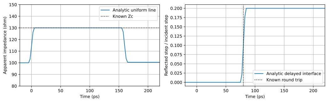
3. Understand TDR on a known line before interpreting EM data
For an ideal line of characteristic impedance \(Z_c\), one-way delay \(\tau\), and reference impedance \(Z_r\), define \(\theta=j2\pi f\tau\). Its transmission matrix is
With \(q=A+B/Z_r+C Z_r+D\), \(S_{11}=(A+B/Z_r-C Z_r-D)/q\) and \(S_{21}=2/q\). We use this independent analytic model to check the time transform. A mismatched line is necessary: a matched line alone would not test impedance recovery.
The transform needs a uniform frequency grid including DC (zero frequency). For EM data beginning at \(\Delta f\), we add a real DC reflection coefficient by linear extrapolation of the lowest two real samples; the imaginary DC value is zero for a real impulse response. This is an assumption about missing low-frequency behavior, not a Palace DC solve. We also compare a constant extrapolation.
A Hamming window reduces ringing from the frequency cutoff but broadens events. The sampling interval is approximately \(1/(2f_{max})\) and the periodic time span is \(1/\Delta f\). scikit-rf centers that interval around zero. Zero padding gives a smoother display, not additional bandwidth. We use \(2/f_{max}\) as a conservative working event-separation scale and verify errors on analytic examples.
For reflected step amplitude \(\rho(t)\),
This is an apparent impedance for our lossy coupled device. It need not equal local characteristic impedance, especially after multiple reflections arrive. Other mixed-mode ports remain terminated at their reference impedances.
The 250 MHz frequency step was selected after checking DC extrapolation on the analytic line. A 500 MHz step gave about 3.1% impedance error with the same linear DC policy; the finer grid meets the 2% analytic criterion without changing it. At 200 GHz, a constant-DC alternative shifts the analytic step by about 2.4 ps (and by about 19 ps at 25 GHz). These policy-dependent shifts limit timing claims.
F_ANALYTIC = np.arange(801) * 0.25e9
bandwidth = F_ANALYTIC[-1]
resolution = 2 / bandwidth
zc, delay, zref = 130.0, 80e-12, 100.0

uniform = line_network(F_ANALYTIC, zc, delay, zref)
t, _, z = tdr(F_ANALYTIC, uniform.s[:, 0, 0], zref)
plateau = (t > 4 * resolution) & (t < 2 * delay - 4 * resolution)
assert plateau.any(), "Increase bandwidth or analytic line length"
z_estimate = np.median(z[plateau])

# First transmitted impulse arrives at the one-way delay.
t_imp, impulse = uniform.s21.impulse_response(window="hamming", bandpass=False)
tau_estimate = t_imp[np.argmax(np.abs(impulse))]
assert abs(z_estimate / zc - 1) < 0.02
assert abs(tau_estimate - delay) < resolution

# A matched launch line ending in 150 ohms gives a delayed reflection.
interface_delay = 40e-12
interface_gamma = (150 - zref) / (150 + zref)
interface_s11 = interface_gamma * np.exp(-4j * np.pi * F_ANALYTIC * interface_delay)
t_gap, r_gap, _ = tdr(F_ANALYTIC, interface_s11, zref)
arrival = t_gap[np.argmin(np.abs(r_gap - interface_gamma / 2))]
assert abs(arrival - 2 * interface_delay) < resolution

# Exercise the DC reconstruction used for real runs, with known DC withheld.
t_ext, _, z_ext = tdr(F_ANALYTIC[1:], uniform.s[1:, 0, 0], zref)
assert abs(np.median(z_ext[plateau]) / zc - 1) < 0.02

analytic_report = pd.DataFrame(
    [
        {
            "check": "uniform impedance",
            "expected": zc,
            "obtained": z_estimate,
            "unit": "ohm",
        },
        {
            "check": "one-way delay",
            "expected": delay * 1e12,
            "obtained": tau_estimate * 1e12,
            "unit": "ps",
        },
        {
            "check": "interface round trip",
            "expected": 2 * interface_delay * 1e12,
            "obtained": arrival * 1e12,
            "unit": "ps",
        },
    ]
)
show(analytic_report)
fig, axes = plt.subplots(1, 2, figsize=(11, 3.5))
axes[0].plot(t * 1e12, z, label="Analytic uniform line")
axes[0].axhline(zc, color="k", ls=":", label="Known Zc")
axes[0].set(
    xlim=(-20, 220),
    ylim=(80, 150),
    xlabel="Time (ps)",
    ylabel="Apparent impedance (ohm)",
)
axes[1].plot(t_gap * 1e12, r_gap, label="Analytic delayed interface")
axes[1].axvline(2 * interface_delay * 1e12, color="k", ls=":", label="Known round trip")
axes[1].set(
    xlim=(-20, 220), xlabel="Time (ps)", ylabel="Reflected step / incident step"
)
for ax in axes:
    ax.grid()
    ax.legend()
fig.tight_layout()
| check | expected | obtained | unit | |
|---|---|---|---|---|
| 0 | uniform impedance | 130.0 | 130.000000 | ohm |
| 1 | one-way delay | 80.0 | 79.950031 | ps |
| 2 | interface round trip | 80.0 | 79.950031 | ps |
4. A generic geometry builder
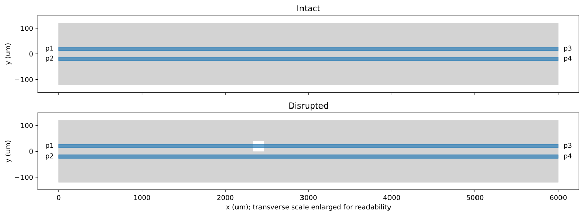
Our two traces sit above a rectangular ground plane. We remove a rectangular interior slot beneath signal A, leaving metal paths around every side. In the intact layout the exchange A ↔ B is a symmetry. The offset slot breaks this symmetry; a centered slot would not necessarily create differential/common-mode conversion.
Dimensions below are initial experiment choices, not an optimized or foundry-qualified interconnect. The 6 mm line and 200 GHz upper frequency are chosen to separate launch, slot, and far-end events. A 120 µm slot may appear as one broadened event: we seek its location, not resolution of both edges.
@dataclass(frozen=True)
class Geometry:
    length: float = 6000.0
    width: float = 14.0
    separation: float = 40.0  # signal center-to-center distance
    ground_width: float = 240.0
    gap_x: float = 2400.0  # slot center, measured from near reference plane
    gap_length: float = 120.0
    gap_y: float = 20.0
    gap_width: float = 36.0


GEO = Geometry()


def make_interconnect(g, signal_layer, return_layer, gap=False):
    if min(g.length, g.width, g.separation, g.ground_width) <= 0:
        raise ValueError("Geometry dimensions must be positive")
    if g.separation <= g.width or g.ground_width <= g.separation + g.width:
        raise ValueError("Signals must be disjoint and fit above the ground")
    c = gf.Component()
    for y, near, far in [
        (g.separation / 2, "p1", "p3"),
        (-g.separation / 2, "p2", "p4"),
    ]:
        c.add_polygon(
            [
                (0, y - g.width / 2),
                (g.length, y - g.width / 2),
                (g.length, y + g.width / 2),
                (0, y + g.width / 2),
            ],
            layer=signal_layer,
        )
        c.add_port(
            name=near,
            center=(0, y),
            width=g.width,
            orientation=180,
            layer=signal_layer,
            port_type="electrical",
        )
        c.add_port(
            name=far,
            center=(g.length, y),
            width=g.width,
            orientation=0,
            layer=signal_layer,
            port_type="electrical",
        )
    dbu = c.kcl.dbu

    def box(x0, y0, x1, y1):
        return gf.kdb.Box(*(round(v / dbu) for v in (x0, y0, x1, y1)))

    ground = gf.kdb.Region(box(0, -g.ground_width / 2, g.length, g.ground_width / 2))
    if gap:
        x0, x1 = g.gap_x - g.gap_length / 2, g.gap_x + g.gap_length / 2
        y0, y1 = g.gap_y - g.gap_width / 2, g.gap_y + g.gap_width / 2
        if not (
            0 < x0 < x1 < g.length
            and -g.ground_width / 2 < y0 < y1 < g.ground_width / 2
        ):
            raise ValueError("Slot must be strictly inside the ground plane")
        ground -= gf.kdb.Region(box(x0, y0, x1, y1))
    ground.merge()
    if ground.count() != 1:
        raise ValueError("Ground must remain one connected polygon")
    c.add_polygon(ground, layer=return_layer)
    return c


def show_layout(g):
    fig, axes = plt.subplots(2, 1, figsize=(12, 4.5), sharex=True)
    for ax, gap, name in zip(axes, [False, True], ["Intact", "Disrupted"], strict=True):
        ax.add_patch(
            Rectangle(
                (0, -g.ground_width / 2),
                g.length,
                g.ground_width,
                color="lightgray",
                label="Return plane (lower layer)",
            )
        )
        if gap:
            ax.add_patch(
                Rectangle(
                    (g.gap_x - g.gap_length / 2, g.gap_y - g.gap_width / 2),
                    g.gap_length,
                    g.gap_width,
                    color="white",
                    hatch="//",
                )
            )
        for y, near, far in [
            (g.separation / 2, "p1", "p3"),
            (-g.separation / 2, "p2", "p4"),
        ]:
            ax.add_patch(
                Rectangle(
                    (0, y - g.width / 2),
                    g.length,
                    g.width,
                    color="tab:blue",
                    alpha=0.65,
                )
            )
            ax.text(-60, y, near, ha="right", va="center")
            ax.text(g.length + 60, y, far, va="center")
        ax.set(
            xlim=(-250, g.length + 250), ylim=(-150, 150), ylabel="y (um)", title=name
        )
    axes[-1].set_xlabel("x (um); transverse scale enlarged for readability")
    fig.tight_layout()


show_layout(GEO)
5. Select IHP layers and declare the physical model
This is the PDK-specific section. The generic builder uses the resolved GDS layer numbers; the solver uses the resolved vertical extents and materials.
The PDK-authoritative branch's IHP overlay supplies missing bulk dielectric regions
and via roles. Here we explicitly replace its ild background with oxide from
\(z=0\) to the declared passivation, and add 180 µm of silicon below \(z=0\).
Passivation comes from the overlay/PDK. No new via geometry is needed for these
interlayer port sheets.
We use the registry's metal and dielectric properties and explicitly set silicon \(\epsilon_r=11.7\), conductivity \(\sigma=10\ \mathrm{S/m}\), and dielectric loss tangent zero (conductivity still causes loss). These are tutorial modeling assumptions, not certified IHP RF substrate parameters. The 180 µm truncation and outer absorbing boundary require sensitivity checks for quantitative substrate-mediated coupling. Inspect the tables before drawing process conclusions.
Aluminum uses the registry's standard conductivity, \(3.77\times10^7\) S/m, through finite-thickness conductivity boundaries. Its attached material-model metadata lists a frequency-validity ceiling of 100 GHz. This tutorial explicitly continues the constant-conductivity assumption to 200 GHz for the TDR bandwidth study. Numerical mesh convergence does not validate that material extrapolation or provide measured foundry data.
from ihp import PDK

PDK.activate()
IHP_REVISION = "d119d9ce0e9ad3092654a1cc9e1d0e18c1d6618f"
initial_stack = resolve_layer_stack(pdk=PDK)
SIGNAL_KEY, RETURN_KEY = "topmetal2", "metal1"
SIGNAL_LAYER = initial_stack.layers[SIGNAL_KEY].gds_layer
RETURN_LAYER = initial_stack.layers[RETURN_KEY].gds_layer
BULK = [
    {
        "name": "ild",
        "material": "sio2",
        "zmin": 0.0,
        "zmax": initial_stack.layers["passiv"].zmin,
    },
    {"name": "substrate", "material": "silicon", "zmin": -180.0, "zmax": 0.0},
]
MATERIAL_OVERRIDES = {
    "silicon": {
        "material_type": "semiconductor",
        "permittivity": 11.7,
        "conductivity": 10.0,
        "loss_tangent": 0.0,
    },
}
components = {
    name: make_interconnect(GEO, SIGNAL_LAYER, RETURN_LAYER, gap)
    for name, gap in [("intact", False), ("disrupted", True)]
}
resolved = resolve_layer_stack(components["intact"], pdk=PDK, dielectrics=BULK)
show(pd.DataFrame([asdict(resolved.layers[k]) for k in (SIGNAL_KEY, RETURN_KEY)]))
show(pd.DataFrame([asdict(d) for d in resolved.dielectrics]))
show(pd.DataFrame.from_dict(dict(resolved.materials), orient="index"))
show(pd.DataFrame.from_dict(MATERIAL_OVERRIDES, orient="index"))
print("Overlay:", resolved.overlay)
print("Reference planes: x=0 and x=", GEO.length, "um; no de-embedding")
| key | declared_name | gds_layer | material | material_properties | zmin | zmax | thickness | sidewall_angle | mesh_order | layer_type | drawn | |
|---|---|---|---|---|---|---|---|---|---|---|---|---|
| 0 | topmetal2 | None | (134, 0) | alcu_sg13g2_topmetal2 | {'conductivity': 30300000.0} | 11.03 | 14.03 | 3.00 | 0.0 | 28 | conductor | True |
| 1 | metal1 | None | (8, 0) | alcu_sg13g2_metal1 | {'conductivity': 21640000.0} | 0.84 | 1.26 | 0.42 | 0.0 | 14 | conductor | True |
| name | material | material_properties | zmin | zmax | source | |
|---|---|---|---|---|---|---|
| 0 | passivation | sin | {'permittivity': 7.5, 'loss_tangent': 0.001, '... | 14.03 | 15.93 | explicit |
| 1 | ild | sio2 | {'conductivity': 0.0, 'permittivity': 4.1} | 0.00 | 14.03 | explicit |
| 2 | substrate | silicon | {'conductivity': 2.0, 'permittivity': 11.9} | -180.00 | 0.00 | explicit |
| conductivity | permittivity | dispersion_models | loss_tangent | |
|---|---|---|---|---|
| si | 2.0 | 11.9 | [{'type': 'cauchy', 'axis': None, 'sellmeier_t... | NaN |
| sin | NaN | 7.5 | [{'type': 'sellmeier', 'axis': None, 'sellmeie... | 0.001 |
| sio2 | 0.0 | 4.1 | NaN | NaN |
| poly_si | 100000.0 | NaN | [{'type': 'constant', 'axis': None, 'sellmeier... | NaN |
| TiN | 5000000.0 | NaN | [{'type': 'constant', 'axis': None, 'sellmeier... | NaN |
| sg13g2_cont | 2390000.0 | NaN | NaN | NaN |
| alcu_sg13g2_metal1 | 21640000.0 | NaN | NaN | NaN |
| tungsten_sg13g2_via1 | 1660000.0 | NaN | NaN | NaN |
| alcu_sg13g2_metal2 | 23190000.0 | NaN | NaN | NaN |
| tungsten_sg13g2_via2 | 1660000.0 | NaN | NaN | NaN |
| alcu_sg13g2_metal3 | 23190000.0 | NaN | NaN | NaN |
| tungsten_sg13g2_via3 | 1660000.0 | NaN | NaN | NaN |
| alcu_sg13g2_metal4 | 23190000.0 | NaN | NaN | NaN |
| tungsten_sg13g2_via4 | 1660000.0 | NaN | NaN | NaN |
| alcu_sg13g2_metal5 | 23190000.0 | NaN | NaN | NaN |
| sg13g2_mim | 500000.0 | NaN | NaN | NaN |
| sg13g2_vmim | 2191000.0 | NaN | NaN | NaN |
| tungsten_sg13g2_topvia1 | 2191000.0 | NaN | NaN | NaN |
| alcu_sg13g2_topmetal1 | 27800000.0 | NaN | NaN | NaN |
| tungsten_sg13g2_topvia2 | 3143000.0 | NaN | NaN | NaN |
| alcu_sg13g2_topmetal2 | 30300000.0 | NaN | NaN | NaN |
| silicon | 2.0 | 11.9 | NaN | NaN |
| material_type | permittivity | conductivity | loss_tangent | |
|---|---|---|---|---|
| silicon | semiconductor | 11.7 | 10.0 | 0.0 |
Overlay: IHP
Reference planes: x=0 and x= 6000.0 um; no de-embedding
6. Configure the solver through PDK-independent inputs
We use lumped terminal ports: vertical sheets from the return layer to each
signal, referenced to 50 Ω. Set excited=True on all four; Palace assigns separate
excitation IDs. We inspect the generated JSON before running.
The executed dense profile uses first-order finite elements with an 8 µm refined
mesh size. The original second-order, 6 µm profile is retained as FULL_SETTINGS,
but its full-band direct solve exceeded the practical memory budget. The recorded
results are exploratory; the final section quantifies the failed convergence checks. Finite-thickness metal
geometry is retained (planar_conductors=False); the generated Palace conductivity
boundaries and material tables should be inspected with the mesh. The airbox and
substrate are part of the physical model, not merely display padding.
The AWS CPW example motivates a launch-refinement check and comparison of adaptive
frequency sweeps with direct solves. Weak crosstalk may need much tighter accuracy
than through transmission. Here adaptive_tol=1e-5 is a starting choice, not a
certified bound on any S-parameter. Direct anchor solves use adaptive_tol=0.
Local execution uses the MUMPS direct solver with relative linear tolerance
1e-8. A pilot benchmark found this substantially faster than the default
iterative preconditioner for these long thin structures. This changes the linear
algebra, not the physical geometry; solver selection and tolerance are recorded
in the experiment settings. Each completed run retains solver.log.
Linear controls come from the public solver API (sim.solver.linear), so they
survive local and cloud config regeneration without a notebook-local subclass.
Future local runs allow up to five correction iterations; archived dense runs
used the original one-iteration MUMPS setting. Archived data are never silently
replaced with corrected values.
MUMPS is the sparse direct-factorization backend. Palace uses that factorization inside generalized minimal residual (GMRES), an iterative linear solver. A preconditioner is an auxiliary, easier-to-solve matrix that helps GMRES; its approximation must not be confused with the physical Maxwell operator. Every accepted field solve must still meet the residual tolerance for the full complex system. Message Passing Interface (MPI) coordinates worker processes; OpenMP supplies CPU threads within each process.
@dataclass(frozen=True)
class Settings:
    fmin: float = 0.25e9
    fmax: float = 200e9
    points: int = 800
    adaptive_tol: float = 1e-5
    refined_um: float = 6.0
    max_um: float = 100.0
    linear_solver: str = "MUMPS"
    linear_tolerance: float = 1e-8
    linear_max_iterations: int = 5
    real_preconditioner: bool = False
    order: int = 2
    air_um: float = 150.0


FULL_SETTINGS = Settings()
# Resource-bounded profile used for the recorded dense comparison.
BASE = replace(FULL_SETTINGS, order=1, refined_um=8.0, max_um=100.0)


def configure_sim(
    component, stack, signal_key, return_key, settings, outdir, material_overrides=None
):
    if signal_key == return_key or not {signal_key, return_key} <= set(stack.layers):
        raise ValueError(
            "Select distinct signal and return layers present in the stack"
        )
    if stack.layers[signal_key].z_bounds[0] <= stack.layers[return_key].z_bounds[1]:
        raise ValueError("This interlayer example requires signal above return")
    sim = DrivenSim()
    sim.set_output_dir(str(outdir))
    sim.set_geometry(component)
    sim.set_stack(build_palace_layer_stack(stack))
    for name, properties in (material_overrides or {}).items():
        sim.set_material(name, **properties)
    sim.set_airbox(
        margin_x=settings.air_um,
        margin_y=settings.air_um,
        z_above=settings.air_um,
        z_below=settings.air_um,
    )
    for name in PORTS:
        sim.add_port(
            name,
            from_layer=return_key,
            to_layer=signal_key,
            geometry="interlayer",
            impedance=Z_SE,
            excited=True,
        )
    sim.set_driven(
        fmin=settings.fmin,
        fmax=settings.fmax,
        num_points=settings.points,
        scale="linear",
        adaptive_tol=settings.adaptive_tol,
        adaptive_max_samples=80,
        reference_impedance=Z_SE,
    )
    sim.solver.order = settings.order
    sim.solver.linear.solver_type = settings.linear_solver
    sim.solver.linear.tolerance = settings.linear_tolerance
    sim.solver.linear.max_iterations = settings.linear_max_iterations
    sim.solver.linear.pc_mat_real = settings.real_preconditioner
    sim.solver.linear.complex_coarse_solve = not settings.real_preconditioner
    return sim


# Planning estimate only: actual delay is extracted from the solved baseline.
v_estimate = 1.5e8
frequency_step = (BASE.fmax - BASE.fmin) / (BASE.points - 1)
print(
    f"df={frequency_step / 1e9:g} GHz; periodic time span={1 / frequency_step * 1e12:g} ps"
)
print(
    f"Approximate sampling={1 / (2 * BASE.fmax) * 1e12:g} ps; "
    f"working resolution={2 / BASE.fmax * 1e12:g} ps"
)
print(f"Estimated gap round trip={2 * GEO.gap_x * 1e-6 / v_estimate * 1e12:g} ps")
df=0.25 GHz; periodic time span=4000 ps
Approximate sampling=2.5 ps; working resolution=10 ps
Estimated gap round trip=32 ps
7. Run or reload complete experiments
preview leaves the expensive stages unexecuted. In local/cloud mode, matching
completed runs are reused only when their manifest and data hash match. A different
geometry, mesh setting, dependency version, or stack produces a different directory.
load requires a previously saved matching result. Partial or failed solves are
recorded with their status and are never treated as completed results.
The raw Palace files remain in the run directory. A compact NPZ (NumPy archive)
contains the complete network; a JSON manifest records its provenance. A Touchstone
.s4p file allows importing the network in other RF tools. No symmetry completion
is used. Reference impedances are read from results, not relabeled during export.
recorded loads the 8 µm first-order pair, checking data hashes, geometry, and
key settings. Original solver warnings and the detailed run tables are retained in
the private lab and the archived logs. A completed data archive is not itself a
validation certificate.
def load_recorded_case(label):
    candidates = []
    for path in OUTPUT.glob(label + "-*"):
        manifest_file = path / "manifest.json"
        if manifest_file.exists():
            manifest = json.loads(manifest_file.read_text())
            if manifest.get("status") == "complete":
                candidates.append((path, manifest))
    if not candidates:
        return None, None, None
    if len(candidates) != 1:
        raise ValueError(f"Ambiguous recorded case {label}; select an explicit archive")
    directory, manifest = candidates[0]
    data_path = directory / "network.npz"
    if hashlib.sha256(data_path.read_bytes()).hexdigest() != manifest["sha256"]:
        raise ValueError(f"Data hash mismatch for {label}")
    with np.load(data_path, allow_pickle=False) as saved:
        net = rf.Network(f=saved["f"], s=saved["s"], z0=saved["z0"], f_unit="Hz")
        net.port_names = saved["ports"].tolist()
    check_network(net, n_ports=4)
    return net, manifest, directory


def json_text(value):
    return json.dumps(value, sort_keys=True, indent=2, default=str)


def stack_record(stack):
    return {
        "pdk": stack.pdk_name,
        "overlay": stack.overlay,
        "notes": list(stack.notes),
        "layers": {k: asdict(v) for k, v in stack.layers.items()},
        "dielectrics": [asdict(d) for d in stack.dielectrics],
        "materials": dict(stack.materials),
    }


def validate_generated_config(config):
    ports = config["Boundaries"]["LumpedPort"]
    ids = [p.get("Excitation") for p in ports]
    if (
        len(ports) != 4
        or any(type(i) is not int for i in ids)
        or set(ids) != {1, 2, 3, 4}
    ):
        raise ValueError(f"Expected four independent excitations, got {ids}")
    if not all(np.isclose(p["R"], Z_SE) for p in ports):
        raise ValueError("Generated port impedances do not match the experiment")


def run_case(label, geometry, gap, settings, bulk=BULK):
    if EXECUTION == "recorded":
        recorded_label = {
            "intact": "refine8-intact",
            "disrupted": "refine8-disrupted",
        }.get(label)
        if recorded_label is None:
            return None  # The full proposed convergence suite was not completed.
        net, manifest, _ = load_recorded_case(recorded_label)
        if net is not None:
            if manifest["spec"]["geometry_um"] != asdict(geometry):
                raise ValueError("Recorded geometry differs from the tutorial controls")
            for key in (
                "fmin",
                "fmax",
                "points",
                "order",
                "refined_um",
                "max_um",
                "air_um",
            ):
                if manifest["spec"]["settings"][key] != getattr(settings, key):
                    raise ValueError(f"Recorded setting differs: {key}")
        return net
    component = make_interconnect(geometry, SIGNAL_LAYER, RETURN_LAYER, gap)
    stack = resolve_layer_stack(component, pdk=PDK, dielectrics=bulk)
    spec = {
        "schema": 1,
        "label": label,
        "geometry_um": asdict(geometry),
        "gap": gap,
        "settings": asdict(settings),
        "stack": stack_record(stack),
        "material_overrides": MATERIAL_OVERRIDES,
        "versions": VERSIONS,
        "gsim_revision": GSIM_REVISION,
        "ihp_source_revision": IHP_REVISION,
        "ihp_install": IHP_INSTALL,
        "palace_version": PALACE_VERSION,
        "ports": list(PORTS),
        "pairs": PAIRS,
        "z_se_ohm": Z_SE,
        "reference_planes_um": [0, geometry.length],
        "tdr": {"dc": "linear-real", "window": "hamming", "pad": 0},
    }
    signature = hashlib.sha256(json_text(spec).encode()).hexdigest()[:16]
    directory = OUTPUT / f"{label}-{signature}"
    manifest_path, data_path = directory / "manifest.json", directory / "network.npz"
    if EXECUTION == "preview":
        return None
    if manifest_path.exists() and data_path.exists():
        manifest = json.loads(manifest_path.read_text())
        if manifest.get("status") == "complete":
            if json_text(manifest["spec"]) != json_text(spec):
                raise ValueError("Manifest mismatch")
            if hashlib.sha256(data_path.read_bytes()).hexdigest() != manifest["sha256"]:
                raise ValueError("Saved network hash mismatch")
            with np.load(data_path, allow_pickle=False) as saved:
                net = rf.Network(
                    f=saved["f"], s=saved["s"], z0=saved["z0"], f_unit="Hz"
                )
                net.port_names = saved["ports"].tolist()
            check_network(net, n_ports=4)
            return net
    if EXECUTION == "load":
        raise FileNotFoundError(f"No completed matching run in {directory}")
    directory.mkdir(parents=True, exist_ok=True)
    manifest = {"status": "incomplete", "spec": spec}
    manifest_path.write_text(json_text(manifest))
    try:
        sim = configure_sim(
            component,
            stack,
            SIGNAL_KEY,
            RETURN_KEY,
            settings,
            directory,
            MATERIAL_OVERRIDES,
        )
        sim.mesh(
            preset="default",
            refined_mesh_size=settings.refined_um,
            max_mesh_size=settings.max_um,
            planar_conductors=False,
            fmax=settings.fmax,
            threads=1,
            surface_threads=1,
        )
        config_path = sim.write_config()
        config = json.loads(Path(config_path).read_text())
        validate_generated_config(config)
        run_logger = logging.getLogger("gsim.palace.base")
        log_handler = logging.FileHandler(directory / "solver.log")
        previous_level = run_logger.level
        run_logger.setLevel(logging.INFO)
        run_logger.addHandler(log_handler)
        try:
            if EXECUTION == "local":
                result = sim.run_local(
                    palace_executable=PALACE_EXECUTABLE,
                    num_processes=LOCAL_PROCESSES,
                    num_threads=2,
                )
            else:
                result = sim.run(parent_dir=directory, check_cache=True)
        finally:
            run_logger.removeHandler(log_handler)
            log_handler.close()
            run_logger.setLevel(previous_level)
        if EXECUTION == "cloud":
            downloaded_logs = sorted(
                path
                for path in directory.glob("sim-data-*/**/*.log")
                if path.name in {"palace.log", "stdout.log", "output.log"}
            )
            if len(downloaded_logs) != 1:
                raise RuntimeError(
                    f"Expected one downloaded Palace solver log, found {len(downloaded_logs)}"
                )
            shutil.copyfile(downloaded_logs[0], directory / "solver.log")
            manifest["cloud_solver_log"] = str(
                downloaded_logs[0].relative_to(directory)
            )
        from gsim.palace.validation import validate_solution

        evidence = validate_solution(
            (directory / "solver.log").read_text(),
            estimator_disabled=config["Solver"]["Linear"].get("EstimatorMaxIts") == 0,
            expected_excitations=[1, 2, 3, 4] if settings.adaptive_tol > 0 else [],
            exit_code=0 if EXECUTION == "local" else None,
        )
        manifest["solver_evidence"] = asdict(evidence)
        if evidence.core.status != "passed":
            raise RuntimeError(
                f"Palace solver convergence was {evidence.core.status}; "
                "archive remains incomplete"
            )
        net = complete_network(result, ports=PORTS, z_se=Z_SE)
        target_f = np.linspace(settings.fmin, settings.fmax, settings.points)
        np.testing.assert_allclose(net.f, target_f, rtol=1e-8, atol=1)
        np.savez_compressed(
            data_path, f=net.f, s=net.s, z0=net.z0, ports=np.array(net.port_names)
        )
        net.write_touchstone(filename=str(directory / "network"))
        manifest.update(
            status="complete",
            sha256=hashlib.sha256(data_path.read_bytes()).hexdigest(),
            config=str(config_path),
        )
        manifest_path.write_text(json_text(manifest))
    except Exception as exc:
        manifest.update(status="failed", error=f"{type(exc).__name__}: {exc}")
        manifest_path.write_text(json_text(manifest))
        raise
    else:
        return net


networks = {
    label: run_case(label, GEO, gap, BASE)
    for label, gap in [("intact", False), ("disrupted", True)]
}
EM_READY = all(net is not None for net in networks.values())
print(
    "Base EM runs complete."
    if EM_READY
    else "EM results INCOMPLETE: preview only; analytic checks are not EM validation."
)
EM results INCOMPLETE: preview only; analytic checks are not EM validation.
8. Read the frequency-domain results
We plot \(20\log_{10}|S|\) (dB). The display floor is −140 dB; it is not a numerical accuracy claim. Each mixed-mode panel shows all four entries in its 2×2 block.
A reciprocal passive network with real power-wave references should have \(S\approx S^T\) and largest singular value \(\sigma_{max}(S)\leq1\). Deviations are useful diagnostics, not proof of physical correctness or a replacement for mesh convergence. All 16 entries must be independently available before these checks.
def db(value):
    return 20 * np.log10(np.maximum(np.abs(value), 1e-7))


if EM_READY:
    mixed = {label: mixed_mode(net)[1] for label, net in networks.items()}
    fig, axes = plt.subplots(2, 2, figsize=(11, 7), sharex=True)
    for ax, (title, i, j) in zip(
        axes.flat,
        [
            ("Reflection S11", 0, 0),
            ("Transmission S31", 2, 0),
            ("NEXT S21", 1, 0),
            ("FEXT S41", 3, 0),
        ],
        strict=True,
    ):
        for label, net in networks.items():
            ax.plot(net.f / 1e9, db(net.s[:, i, j]), label=label)
        ax.set(title=title, xlabel="Frequency (GHz)", ylabel="Magnitude (dB)")
        ax.grid()
        ax.legend()
    fig.tight_layout()

    fig, axes = plt.subplots(2, 2, figsize=(12, 8), sharex=True)
    colors = ["tab:blue", "tab:orange", "tab:green", "tab:red"]
    for ax, (block, row, col) in zip(
        axes.flat, [("dd", 0, 0), ("dc", 0, 2), ("cd", 2, 0), ("cc", 2, 2)], strict=True
    ):
        for label, net in mixed.items():
            style = "-" if label == "intact" else "--"
            for k, (i, j) in enumerate([(0, 0), (0, 1), (1, 0), (1, 1)]):
                ax.plot(
                    net.f / 1e9,
                    db(net.s[:, row + i, col + j]),
                    ls=style,
                    color=colors[k],
                    label=f"{label}: S{block}{i + 1}{j + 1}",
                )
        ax.set(title=f"S{block}", xlabel="Frequency (GHz)", ylabel="Magnitude (dB)")
        ax.grid()
        ax.legend(fontsize=7, ncol=2)
    fig.tight_layout()
    show(
        pd.DataFrame(
            [
                {
                    "case": label,
                    "max |S-S^T|": np.max(np.abs(net.s - net.s.transpose(0, 2, 1))),
                    "max singular value": np.linalg.svd(net.s, compute_uv=False).max(),
                    "max mode conversion (linear)": max(
                        np.abs(mixed[label].s[:, :2, 2:]).max(),
                        np.abs(mixed[label].s[:, 2:, :2]).max(),
                    ),
                }
                for label, net in networks.items()
            ]
        )
    )
else:
    print("Frequency-domain EM plots pending completed runs.")
Frequency-domain EM plots pending completed runs.
9. Locate the return-path interruption with TDR
We estimate the baseline's differential propagation delay from the phase slope: \(\tau_g=-d\arg(S_{dd21})/d\omega\). This includes the launches and may vary with frequency. Its median is a timing estimate, not an independently known material velocity. A uniform-path estimate of the gap echo is \(t_{gap}\approx2\tau_g x_{gap}/L\).
Overlay intact/disrupted reflected steps and apparent impedances, then examine the difference in reflected steps. Estimate its first half-peak excursion within a fixed interior time gate that excludes the launches and far-end reflection. Use the same gate for both slot locations; the expected arrival is used only to assess the result, never to steer the search. Multiple interior reflections can still make this estimator ambiguous. A moved-slot experiment below provides a stronger check.
We also vary DC extrapolation, window, and upper bandwidth. A feature that moves substantially under those choices is not yet a reliably located discontinuity.
if EM_READY:
    tau = differential_delay(mixed["intact"])
    predicted = 2 * tau * GEO.gap_x / GEO.length
    time_resolution = 2 / BASE.fmax
    print(f"Baseline median one-way group delay: {tau * 1e12:.2f} ps")
    print(
        f"Estimated slot round trip: {predicted * 1e12:.2f} ps (launch delay included)"
    )
    if min(predicted, 2 * tau - predicted) < 3 * time_resolution:
        print(
            "Resolution warning: extend the line or bandwidth before claiming localization."
        )
    fig, axes = plt.subplots(1, 2, figsize=(12, 4))
    for label, net in mixed.items():
        t, rho, z = tdr(net.f, net.s[:, 0, 0], 2 * Z_SE)
        axes[0].plot(t * 1e12, rho, label=label)
        axes[1].plot(t * 1e12, z, label=label)
    for ax in axes:
        ax.axvline(predicted * 1e12, color="k", ls=":", label="Estimated slot arrival")
        ax.set(
            xlim=(
                -2 * time_resolution * 1e12,
                min(3 * tau, 0.4 / frequency_step) * 1e12,
            ),
            xlabel="Time (ps)",
        )
        ax.grid()
        ax.legend()
    axes[0].set_ylabel("Reflected differential step / incident step")
    axes[1].set_ylabel("Apparent differential impedance (ohm)")
    fig.tight_layout()

    t, r_intact, _ = tdr(mixed["intact"].f, mixed["intact"].s[:, 0, 0], 2 * Z_SE)
    _, r_disrupted, _ = tdr(
        mixed["disrupted"].f, mixed["disrupted"].s[:, 0, 0], 2 * Z_SE
    )
    fig_delta, ax_delta = plt.subplots(figsize=(9, 3))
    ax_delta.plot(t * 1e12, r_disrupted - r_intact, label="Disrupted minus intact")
    ax_delta.axvline(
        predicted * 1e12, color="k", ls=":", label="Estimated slot arrival"
    )
    ax_delta.set(
        xlim=(-20, 3 * tau * 1e12),
        xlabel="Time (ps)",
        ylabel="Change in reflected step",
    )
    ax_delta.grid()
    ax_delta.legend()
    fig_delta.tight_layout()

    fig, ax = plt.subplots(figsize=(9, 4))
    net = mixed["disrupted"]
    for window, dc, fraction in [
        ("hamming", "linear", 1),
        ("hamming", "constant", 1),
        ("hann", "linear", 1),
        ("hamming", "linear", 0.5),
    ]:
        count = int(len(net.f) * fraction)
        t, rho, _ = tdr(
            net.f[:count], net.s[:count, 0, 0], 2 * Z_SE, window=window, dc=dc
        )
        ax.plot(
            t * 1e12,
            rho,
            label=f"{window}, DC={dc}, fmax={net.f[count - 1] / 1e9:g} GHz",
        )
    ax.set(
        xlim=(-20, 3 * tau * 1e12),
        xlabel="Time (ps)",
        ylabel="Reflected differential step",
    )
    ax.grid()
    ax.legend()
    fig.tight_layout()
else:
    print("EM TDR and DC/window/bandwidth sensitivity pending completed runs.")
EM TDR and DC/window/bandwidth sensitivity pending completed runs.
10. Convergence status: what is and is not resolved
The device networks in this tutorial are exploratory. A fixed-mesh check of adaptive versus direct frequency points is not a spatial-convergence proof, so the acceptance criteria and the full audit are kept in the companion lab notebook. They are reproduced here as a status summary, not as tutorial code.
The criteria chosen before the EM results were:
- maximum study difference below 0.01 in absolute complex S;
- baseline mode conversion no greater than three times that indicator;
- gap-induced mixed-mode conversion change greater than three times it;
- gap reflection detectable above three times the TDR mesh indicator;
- slot arrival and moved-slot shift agreeing with the propagation estimate within the working time resolution.
| Check | Recorded outcome |
|---|---|
| Spatial convergence | Failed: mesh changes reached about 0.25 in single-ended S and 0.377 in mixed-mode S |
| Compact slot-region check | At 25 GHz on a 1.6 mm device, complete second-order coarse/default four-port networks differed by at most 0.005135 in complex S; the selected coarse settings are in the companion lab. This does not validate the 6 mm device |
| Baseline mode conversion | Fell from about 0.094 to 0.037 on refinement, indicating numerical symmetry breaking |
| Slot conversion change | About 0.052, below the three-times-mesh indicator |
| TDR slot feature | About 1.4% of the incident step, below the 5.4% mesh-variation indicator |
| Element-order check | Incomplete four-port comparison; selected anchors differed by 0.07–0.14 |
Conclusion: the recorded device numbers are useful for the tutorial workflow and for interpreting trends, but they do not establish a converged slot response. See the companion lab notebook for the archived runs and audit code.
11. What can we conclude?
The analytic cells check mixed-mode algebra, port reordering, uniform-line impedance and delay recovery, and a known reflection time. These checks validate the postprocessing on those examples; they do not validate the IHP electromagnetic model.
After the EM runs, use the reported convergence results to decide whether the gap's mode conversion and reflection are resolved. A small symmetry residual is an empirical diagnostic. Apparent TDR impedance includes launch effects, finite bandwidth, loss, coupling, and repeated reflections. The substrate assumptions must be replaced or justified before making claims about fabricated IHP devices.
Useful next experiments are changing trace separation, slot offset, and return width one at a time. A centered slot is a useful symmetry control. Eye diagrams and bit error rate (BER) require transmitter/receiver/noise assumptions and are outside this tutorial's validation claims.
Sources and adaptations
- AWS Palace: crosstalk between coplanar waveguides (CPWs): four-terminal coupling, lumped/wave-port comparisons, mesh/order sensitivity, and checking adaptive sweeps against direct solves. Its sapphire CPW is not our IHP geometry. We do not assume its numerical curves transfer to this stack.
- Palace v0.18.1 CPW configuration: explicit excitation IDs. Our full mixed-mode matrix requires all four excitations.
- PalaceToolkit,
docs/examples/signal_integrity.ipynb: inspiration for a common variant builder, separate mesh/solve/analysis stages, and consistent comparisons. Its bent-antenna geometry and passband OOK (on-off keying) eye/BER model are not used as a TDR algorithm. This notebook does not depend on PalaceToolkit. - scikit-rf mixed-mode conversion and step response.
- scikit-rf TDR tutorial: DC treatment, windowing, and time-resolution considerations.
12. Executed experiments: what the evidence supports
The local run used Palace v0.18.0. Two dense first-order mesh levels (12/150 µm and 8/100 µm refined/background sizes) and nine direct frequency anchors were run for the intact and disrupted return planes. The 6 µm second-order direct run was stopped when host memory reached approximately 55 GiB and swapping began. The initial iterative run was stopped after benchmarking a faster direct solver. Neither stopped run supplies a completed network.
A second-order spot check on the same 12 µm mesh produced one complete excitation column at 25 GHz before that study was stopped. It is adverse evidence about spatial discretization, not a complete four-port validation. The remaining second-order frequencies/excitations and the proposed airbox/substrate sensitivity suite were not completed. Thus the full issue acceptance criteria are not met.
The selected values below distinguish complete matrices, adaptive training convergence, linear residual warnings, direct-sweep agreement, and mesh/order sensitivity. The moved-slot experiment is an empirical timing check on the coarse model. Matching its expected delay cannot establish continuum accuracy when discretization checks fail.
The nine direct-check frequencies are not all on the 250 MHz output grid. Both linear and cubic interpolation comparisons are reported: the former includes a visible interpolation error of its own. These are checks at selected frequencies, not rigorous error bounds over the full band; the endpoints are training points.
13. Interpreting this run
The simulations produced networks, but the discretization checks failed. Agreement between direct and adaptive frequency sweeps tests the frequency approximation on a fixed mesh. Reciprocity and passivity are useful consistency diagnostics. None of these tests establishes accuracy of the spatial finite-element approximation.
The intact-line mesh change alone reaches approximately 0.25 in complex single-ended S, versus the proposed 0.01 criterion. The symmetric baseline's largest cross-mode amplitude falls from 0.094 to 0.037 on refinement, indicating substantial numerical symmetry breaking. On the same coarse mesh, increasing the element order changes the 25 GHz far-end crosstalk from approximately −42.3 to −23.3 dB, or |S41| ≈ 0.0077 to 0.0684. Both are small compared with unit transmission, but the absolute change ≈ 0.061 exceeds the proposed 0.01 complex-S tolerance, and the coupling amplitude changes by about ninefold. Consequently, the slot's crosstalk and conversion effects cannot yet be separated reliably from discretization error. A separate local one-source, 200 GHz terminal/slot-end refinement pilot gave a 0.01916 complex-S change against the same 0.01 target. Its run archive is not committed, so it is reported only as an unverified pilot, not as evidence for the archived four-port study.
The coarse timing experiment is qualitatively consistent: moving the slot by 1.2 mm moves the fixed-gate half-peak arrival from 30.0 to 47.5 ps, a 17.5 ps shift compared with the 16.1 ps estimate from group delay. The approximate Hamming-window resolution is 10 ps. This is an exploratory timing observation, not a demonstrated localization accuracy. The apparent impedance curve is likewise not a converged characteristic impedance measurement.
Numerical values from the finer first-order pair (exploratory)
At 100 GHz, differential transmission \(S_{dd21}\) is −4.204 dB intact and −4.228 dB disrupted. Differential reflection \(S_{dd11}\) is −17.673 dB and −19.758 dB, respectively. The slot therefore does not simply worsen reflection at every frequency: its extra reflected wave interferes with the existing reflections. Single-ended near-end/far-end crosstalk is −27.02/−16.01 dB intact, versus −25.55/−15.79 dB disrupted.
The finer slot-induced reflected-step peak is 0.01428 at 32.48 ps (about 1.43% of the incident step); the apparent-impedance difference there is 2.29 Ω. The coarse peak is approximately 0.01702. The maximum change in either absolute reflected-step curve across meshes is 0.05378. This conservative mesh-variation indicator is larger than the slot feature; it is not a statistical confidence interval or a rigorous bound on the difference.
The largest mixed-mode mesh change is 0.3765, while the slot-induced cross-mode change is 0.05176. Both the absolute 0.01 convergence criterion and the requirement that the effect exceed three times the mesh indicator fail. The saved tables retain these unfavorable checks alongside the timing plots.
What to improve before using these numbers for design
- Establish element-order and mesh convergence at direct frequency anchors first. The partial second-order result is a diagnostic, not a reference solution.
- Use sufficient memory for the full higher-order problem, or establish a scalable iterative-solver configuration. The attempted full second-order direct solve approached 55 GiB host memory and was stopped when swapping began.
- Repeat the dense intact/disrupted pair only after the direct checks settle; then complete the airbox and substrate-depth sensitivity studies.
- Repeat the moved-slot and DC/window/bandwidth checks with the converged spectra. Require the slot-induced change to exceed the measured numerical variation.
All failed checks and stopped runs are retained. These results do not establish that the physical slot has no effect; they establish that this discretization is insufficient to quantify that effect.
Reproducing the tutorial profiles
The public run_case helper in section 7 regenerates the resource-bounded
intact/disrupted pair. Set EXECUTION = "local" or "cloud", choose the Palace
runtime, and keep every manifest, mesh, configuration, and solver log. The
convergence profiles and the aligned-mesh study are in the companion lab notebook.
A fresh run with a changed parameter is a new experiment, not a replacement for an
unfavorable convergence result.