Silicon Traveling-Wave Mach-Zehnder Modulator: from Doping to Bandwidth
A silicon modulator writes an electrical signal onto light. This notebook simulates one end to end, starting from a drawn gdsfactory component and ending with the numbers a designer quotes: modulation efficiency \(V_\pi L\), optical loss, line impedance and electro-optic bandwidth. Everything runs on open-source solvers.
How the device works
- The waveguide is a silicon rib with a PN junction along its centre. Around the junction sits a depletion region, a strip of silicon emptied of free electrons and holes.
- A reverse bias widens that depleted strip. Fewer free carriers means a slightly higher refractive index and a slightly lower absorption: this is the plasma-dispersion effect. The light in the rib therefore picks up a voltage-controlled phase.
- A Mach-Zehnder interferometer turns the phase shift into an intensity change. \(V_\pi L\) is the voltage needed for a \(\pi\) phase shift, times the length it takes; lower is better.
- The effect is weak (\(\Delta n_{eff} \sim 10^{-4}\)), so the phase shifter is millimetres long, which is many RF wavelengths at tens of GHz. The drive electrode is therefore a transmission line running alongside the waveguide, so that the RF wave travels with the light: a traveling-wave modulator. Bandwidth is then set by three things: how well the RF and optical velocities match, how much the RF wave is attenuated along the line, and how well the line is matched to its source and termination.
What the notebook computes
| Step | Question | Solver | Result |
|---|---|---|---|
| 1. Charge | Where are the electrons and holes at each bias? | DEVSIM (drift-diffusion), gsim.tcad |
carrier maps \(n(y,z)\), \(p(y,z)\), junction capacitance \(C(V)\) |
| 2. Carriers | What do those carriers do to the silicon? | closed-form, gsim.common.carriers |
optical \(\Delta n\), \(\Delta\alpha\); RF conductivity \(\sigma\) |
| 3. Optical | How does the guided mode respond? | femwell (FEM mode solver) | \(n_{eff}(V)\), optical loss, \(V_\pi L\) |
| 4. RF | What transmission line does the RF signal see? | femwell | RF index, RF loss, \(Z_0\) versus frequency |
| 5. Device | What does the whole modulator do? | transmission-line model, gsim.common.twmzm |
EO response, 3 dB bandwidth, \(V_\pi\), chirp |
All the physics is solved on the cross-section of the device: the \((y, z)\) plane at \(x = 0\), with the light and the RF wave propagating along \(x\). \(y\) runs across the junction and \(z\) is vertical. Each step is a few lines of plain code calling the gsim building blocks directly, so every setting is in view and can be changed.
Install everything with the two extras:
The device
The example is a depletion-mode phase shifter as foundries build one: a
500 × 220 nm silicon rib on a 90 nm slab, with a lateral PN junction at the
centre of the rib. Going out from the junction on each side, the silicon is
rib | slab | plus | contact:
- the lightly doped core (p 5e17, n 3e17 cm⁻³): the rib half and 0.5 µm of slab beside it. This is where the light is and where the depletion edge moves. Light doping keeps the optical loss down;
- a moderately doped plus region (1e19 cm⁻³, 1 µm wide) that carries the current to the core with little resistance;
- a heavily doped contact region (1e20 cm⁻³, 1 µm wide) under the metal, so the metal-silicon contact is Ohmic.
The doping increases in steps away from the rib because free carriers absorb light: you want them near the metal, where they lower the series resistance, and not near the optical mode. Aluminium, 1 µm thick, lands on each contact region.
These are generic published values for a 220 nm SOI depletion modulator, not any foundry's. The cell below draws each doped region on a layer of its own and builds the layer stack the cross-section is cut from. In your own workflow you bring your own component and layer stack, and everything below stays the same.
The doped silicon is drawn at a constant permittivity. It is given silicon's own dispersion at optical wavelengths as well, so that the group index computed in Step 5 carries material dispersion and not only the waveguide's.
import logging

import gdsfactory as gf
import matplotlib.pyplot as plt
import numpy as np

from gsim.common.cross_section import build_doped_cross_section
from gsim.common.stack.extractor import Layer
from gsim.common.stack.materials import MATERIALS_DB, make_doped_materials

# The mesher's advice on air boxes and absorbing boundaries targets 3D
# driven simulations; it does not apply to these cross-section solves.
logging.getLogger("gsim.palace").setLevel(logging.ERROR)

WAVELENGTH_UM = 1.55
REVERSE_BIASES = np.linspace(0, 2, 11)  # V on the cathode = reverse bias
RF_FREQS_HZ = [1e9, 2e9, 5e9, 10e9, 20e9, 40e9, 60e9, 80e9, 100e9]
LENGTH_UM = 3000.0  # traveling-wave electrode length

CENTER_Y = -20.0  # junction position along y (um)
RIB_HEIGHT, SLAB_HEIGHT = 0.22, 0.09  # um
METAL_THICKNESS = 1.0  # um
# Doped regions from the n-side contact to the p-side one:
# name: (dopant, width um, height um, concentration cm^-3)
REGIONS = {
    "n_contact": ("donor", 1.0, SLAB_HEIGHT, 1e20),
    "n_plus": ("donor", 1.0, SLAB_HEIGHT, 1e19),
    "n_slab": ("donor", 0.5, SLAB_HEIGHT, 3e17),
    "n_rib": ("donor", 0.25, RIB_HEIGHT, 3e17),
    "p_rib": ("acceptor", 0.25, RIB_HEIGHT, 5e17),
    "p_slab": ("acceptor", 0.5, SLAB_HEIGHT, 5e17),
    "p_plus": ("acceptor", 1.0, SLAB_HEIGHT, 1e19),
    "p_contact": ("acceptor", 1.0, SLAB_HEIGHT, 1e20),
}
ELECTRODES = {"n_contact": "cathode_metal", "p_contact": "anode_metal"}

gf.gpdk.PDK.activate()
component = gf.Component()
layers, spans = {}, {}
y = CENTER_Y - sum(width for _, width, _, _ in REGIONS.values()) / 2
for i, (name, (_, width, height, _)) in enumerate(REGIONS.items()):
    spans[name] = (y, y + width)
    rect = component << gf.c.rectangle((10.0, width), layer=(30, i))
    rect.y = y + width / 2
    layers[name] = Layer(
        name=name,
        gds_layer=(30, i),
        zmin=0.0,
        zmax=height,
        thickness=height,
        material=name,
        layer_type="dielectric",
        # The rib and the slab beside it are where the depletion edge moves.
        mesh_resolution="medium" if "plus" in name or "contact" in name else "fine",
    )
    y += width
for i, (region, metal) in enumerate(ELECTRODES.items()):
    y0, y1 = spans[region]
    rect = component << gf.c.rectangle((10.0, y1 - y0), layer=(46, i))
    rect.y = (y0 + y1) / 2
    layers[metal] = Layer(
        name=metal,
        gds_layer=(46, i),
        zmin=SLAB_HEIGHT,
        zmax=SLAB_HEIGHT + METAL_THICKNESS,
        thickness=METAL_THICKNESS,
        material="aluminum",
        layer_type="conductor",
        mesh_resolution="fine",
    )

materials = make_doped_materials([(name, 0.0) for name in REGIONS], permittivity=11.9)
sellmeier = next(
    m for m in MATERIALS_DB["silicon"].dispersion_models if m.type == "sellmeier"
)
for properties in materials.values():
    properties.dispersion_models.append(sellmeier)
stack, _ = build_doped_cross_section(
    component,
    axis="x",
    value=0.0,
    substrate_thickness=2.0,
    doping={"layer_specs": layers, "materials": materials},
    verbose=False,
)

for name, (dopant, _, height, concentration) in REGIONS.items():
    y0, y1 = spans[name]
    print(
        f"{name:10s} y = {y0:7.2f} .. {y1:7.2f} um, {height * 1e3:3.0f} nm tall, "
        f"{dopant:8s} {concentration:.0e} cm^-3"
    )
n_contact  y =  -22.75 ..  -21.75 um,  90 nm tall, donor    1e+20 cm^-3
n_plus     y =  -21.75 ..  -20.75 um,  90 nm tall, donor    1e+19 cm^-3
n_slab     y =  -20.75 ..  -20.25 um,  90 nm tall, donor    3e+17 cm^-3
n_rib      y =  -20.25 ..  -20.00 um, 220 nm tall, donor    3e+17 cm^-3
p_rib      y =  -20.00 ..  -19.75 um, 220 nm tall, acceptor 5e+17 cm^-3
p_slab     y =  -19.75 ..  -19.25 um,  90 nm tall, acceptor 5e+17 cm^-3
p_plus     y =  -19.25 ..  -18.25 um,  90 nm tall, acceptor 1e+19 cm^-3
p_contact  y =  -18.25 ..  -17.25 um,  90 nm tall, acceptor 1e+20 cm^-3
One component, three cross-section windows
Each step meshes only the part of the cross-section its physics needs, its window:
- charge spans the doped silicon from one metal contact to the other, plus 0.5 µm. The oxide far away and the bulk of the electrodes play no role in carrier transport;
- optical is a box of a few µm around the rib, enough to hold the guided mode and its evanescent tails;
- RF keeps the full cross-section of the transmission line, because the RF field fills the whole gap between the electrodes and the space around them.
The depletion edge moves by only tens of nanometres over the bias sweep, so both
the charge mesh and the optical mesh are held to 10 nm across the whole rib
(JUNCTION_BOX), where that edge moves.
DOPED_SPAN = (spans["n_contact"][0], spans["p_contact"][1])
RIB_SPAN = (spans["n_rib"][0], spans["p_rib"][1])
CHARGE_WINDOW = (DOPED_SPAN[0] - 0.5, DOPED_SPAN[1] + 0.5)
OPTICAL_WINDOW = (CENTER_Y - 2.0, CENTER_Y + 2.0)
OPTICAL_WINDOW_Z = (-1.0, RIB_HEIGHT + 1.0)
JUNCTION_BOX = (*RIB_SPAN, 0.0, RIB_HEIGHT, 0.01)  # (y0, y1, z0, z1, size) um

print(f"charge  window: y in {CHARGE_WINDOW} um (doped slab between contacts)")
print(f"optical window: y in {OPTICAL_WINDOW} um, z in {OPTICAL_WINDOW_Z} um")
print(f"rib, held to 10 nm elements: y in {RIB_SPAN} um")
charge  window: y in (-23.25, -16.75) um (doped slab between contacts)
optical window: y in (-22.0, -18.0) um, z in (-1.0, 1.22) um
rib, held to 10 nm elements: y in (-20.25, -19.75) um
A helper to draw each step's mesh
Every step writes its mesh into its own folder under ./tcad-twmzm. The helper
below draws one, with a colour per region, or a colour scale for regions given
a value (used later for conductivity). Metal that a step leaves out of its
mesh shows as a white hole. It is plotting code only; skip it on a first read.
import meshio
from matplotlib.collections import PolyCollection
from matplotlib.colors import LogNorm

REGION_COLORS = {}  # one colour per region name, stable across figures


def plot_cross_section(
    mesh_path,
    *,
    ax,
    title=None,
    values=None,
    label=None,
    xlim=None,
    ylim=None,
):
    """Draw a cross-section mesh, one colour per region or a log colour scale."""
    mesh = meshio.read(mesh_path, file_format="gmsh")
    points = mesh.points[:, :2]
    names = {tag: name for name, (tag, dim) in mesh.field_data.items() if dim == 2}
    triangles = mesh.cells_dict["triangle"]
    tags = mesh.cell_data_dict["gmsh:physical"]["triangle"]

    handles, scalar_polys, scalar_values = [], [], []
    for tag in sorted(set(tags), key=names.get):
        name, polys = names[tag], points[triangles[tags == tag]]
        if values is not None and name in values:
            scalar_polys.extend(polys)
            scalar_values.extend([values[name]] * len(polys))
            continue
        color = REGION_COLORS.setdefault(
            name, plt.get_cmap("tab20")(len(REGION_COLORS) % 20)
        )
        ax.add_collection(
            PolyCollection(
                polys,
                facecolors=color,
                edgecolors="k",
                linewidths=0.1,
                rasterized=True,
            )
        )
        handles.append(plt.Rectangle((0, 0), 1, 1, color=color, label=name))
    if scalar_polys:
        shown = np.maximum(np.asarray(scalar_values, dtype=float), 1e-2)
        coll = PolyCollection(
            scalar_polys,
            array=shown,
            cmap="viridis",
            norm=LogNorm(shown.min(), max(shown.max(), 10 * shown.min())),
            edgecolors="k",
            linewidths=0.1,
            rasterized=True,
        )
        ax.add_collection(coll)
        plt.colorbar(coll, ax=ax, label=label, fraction=0.03)

    ax.autoscale_view()
    ax.set_aspect("equal")
    if xlim is not None:
        ax.set_xlim(xlim)
    if ylim is not None:
        ax.set_ylim(ylim)
    ax.set(xlabel="y (um)", ylabel="z (um)", title=title)
    if handles:
        ax.legend(
            handles=handles,
            fontsize=7,
            ncol=min(len(handles), 6),
            loc="upper center",
            bbox_to_anchor=(0.5, -0.3),
        )
    return ax
Step 1: charge transport (DEVSIM)
gsim.tcad solves the semiconductor equations on the doped silicon: Poisson's
equation for the electrostatic potential, coupled to drift-diffusion continuity
equations for electrons and holes. It does so at every bias of the sweep.
The simulation is configured by physical concern. Every doped region gets its doping profile; each metal landing on a contact region is a contact; every pair of touching doped regions is an interface, the one between the two rib halves being the junction. The oxide around the silicon is declared an insulator: Poisson's equation is solved there too (the potential alone, there are no carriers), so that the capacitance counts the field that fringes around the junction.
The bias is applied to the cathode (the contact on the n side), so a positive voltage is a reverse bias: the regime a depletion modulator is driven in, where almost no current flows and the junction behaves as a voltage-dependent capacitor.
from itertools import pairwise

from gsim import tcad

charge = tcad.Simulation()
charge.geometry(component, stack=stack)
charge.domain(
    plane="x=0",
    window=CHARGE_WINDOW,
    margin_x=2.0,
    margin_y=2.0,
    z_above=1.5,
    z_below=1.0,
)
charge.materials(insulators={"sio2": stack.materials["sio2"]["permittivity"]})
for name, (dopant, _, _, concentration) in REGIONS.items():
    charge.doping.add(
        tcad.StepDoping(
            region=name, dopant_type=dopant, concentration_cm3=concentration
        )
    )
charge.contacts.add(
    name="cathode", semiconductor="n_contact", electrode="cathode_metal"
)
charge.contacts.add(name="anode", semiconductor="p_contact", electrode="anode_metal")
for left, right in pairwise(REGIONS):
    junction = (left, right) == ("n_rib", "p_rib")
    charge.interfaces.add(
        name="junction" if junction else f"{left}_{right}",
        region_a=left,
        region_b=right,
    )
charge.solver(
    mesh_preset="coarse",
    refined_mesh_size_um=0.02,
    max_mesh_size_um=40.0,
    refinement_boxes=[JUNCTION_BOX],
)
charge_mesh = charge.mesh(output_dir="./tcad-twmzm/charge")
Each bias point gives:
- the carrier maps \(n(y,z)\) and \(p(y,z)\), which every later step uses;
- the terminal currents (tiny leakage, in reverse bias);
- the junction capacitance per unit length, from a small-signal AC solve around that bias.
Expect this step to take a minute or two.
sweep = charge.sweep(REVERSE_BIASES, contact="cathode")

for point in sweep.points:
    print(
        f"V = {point.bias_v:4.1f} V:  C = {point.capacitance_f_per_m * 1e12:6.1f} pF/m,"
        f"  I_cathode = {point.currents_a_per_cm['cathode']:+.2e} A/cm"
    )
V =  0.0 V:  C =  392.4 pF/m,  I_cathode = +6.17e-45 A/cm
V =  0.2 V:  C =  361.2 pF/m,  I_cathode = -1.80e-15 A/cm
V =  0.4 V:  C =  337.6 pF/m,  I_cathode = -3.49e-15 A/cm
V =  0.6 V:  C =  319.0 pF/m,  I_cathode = -4.56e-15 A/cm
V =  0.8 V:  C =  303.8 pF/m,  I_cathode = -5.75e-15 A/cm
V =  1.0 V:  C =  290.9 pF/m,  I_cathode = -6.97e-15 A/cm
V =  1.2 V:  C =  279.9 pF/m,  I_cathode = -8.15e-15 A/cm
V =  1.4 V:  C =  270.3 pF/m,  I_cathode = -9.14e-15 A/cm
V =  1.6 V:  C =  261.8 pF/m,  I_cathode = -1.01e-14 A/cm
V =  1.8 V:  C =  254.4 pF/m,  I_cathode = -1.11e-14 A/cm
V =  2.0 V:  C =  247.6 pF/m,  I_cathode = -1.20e-14 A/cm
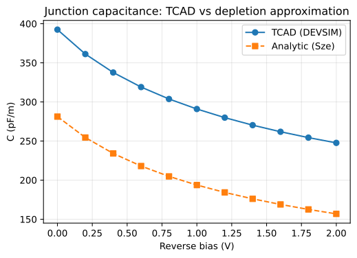
The capacitance falls as the reverse bias grows: the depletion region is the capacitor's dielectric, and it is getting wider.
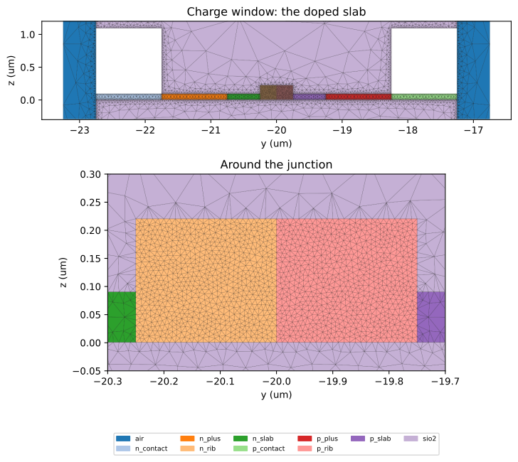
Below is the mesh the charge solve ran on: the eight doped regions between the
two contacts, surrounded by oxide. The electrodes are not part of the
semiconductor problem. They appear as white holes, and the edges where they
touch the silicon are the anode and cathode contacts where the voltage is
applied. At both ends, past the contacts where the drawn component stops, the
window's 0.5 µm margins are air: tcad.Simulation meshes its background as air
and leaves it out of the solve. The close-up shows the 10 nm elements across the
rib.
fig, axes = plt.subplots(2, 1, figsize=(12, 7), height_ratios=(1, 2))
plot_cross_section(
    charge_mesh.mesh_path,
    ax=axes[0],
    title="Charge window: the doped slab",
    ylim=(-0.3, 1.2),
)
axes[0].get_legend().remove()  # the close-up below carries it
plot_cross_section(
    charge_mesh.mesh_path,
    ax=axes[1],
    title="Around the junction",
    xlim=(CENTER_Y - 0.3, CENTER_Y + 0.3),
    ylim=(-0.05, 0.3),
)
plt.tight_layout()
plt.show()
Check: \(C(V)\) against the textbook formula
For an abrupt junction the textbook depletion approximation gives the
depletion width \(W(V)\) in closed form, and the capacitance per unit length is
that of a parallel-plate capacitor, \(C = \varepsilon_{Si}\, h / W(V)\), with \(h\)
the rib height. PNJunctionConfig implements it, and
tcad.compare_capacitance puts it next to the simulated curve.
The simulation sits 100 to 123 pF/m above the formula. The formula is
one-dimensional: it is the path through the depleted silicon alone. The offset
is the field that fringes through the oxide above and below the junction, from
one conducting half of the silicon to the other: a second capacitor in
parallel, whose plates hardly move with the bias, which is why the offset
changes much less than the capacitance itself while the relative deviation
grows along the sweep. Without the oxide
(charge.materials(insulators={})) the solve keeps to the silicon, and the
offset all but disappears.
from gsim.common.stack.pn_junction import PNJunctionConfig

junction = PNJunctionConfig(na_cm3=REGIONS["p_rib"][3], nd_cm3=REGIONS["n_rib"][3])
comparison = tcad.compare_capacitance(junction, sweep, height_um=RIB_HEIGHT)
offset = (comparison.c_tcad_f_per_cm - comparison.c_analytic_f_per_cm) * 1e14
print(f"max relative deviation: {comparison.max_relative_deviation:.1%}")
print(f"offset above the formula: {offset.min():.0f} to {offset.max():.0f} pF/m")

fig, ax = plt.subplots(figsize=(6, 4))
ax.plot(
    comparison.v_reverse, comparison.c_tcad_f_per_cm * 1e14, "o-", label="TCAD (DEVSIM)"
)
ax.plot(
    comparison.v_reverse,
    comparison.c_analytic_f_per_cm * 1e14,
    "s--",
    label="Analytic (Sze)",
)
ax.set_xlabel("Reverse bias (V)")
ax.set_ylabel("C (pF/m)")
ax.set_title("Junction capacitance: TCAD vs depletion approximation")
ax.legend()
ax.grid(alpha=0.3)
plt.show()
max relative deviation: 57.9%
offset above the formula: 91 to 111 pF/m
Carrier maps
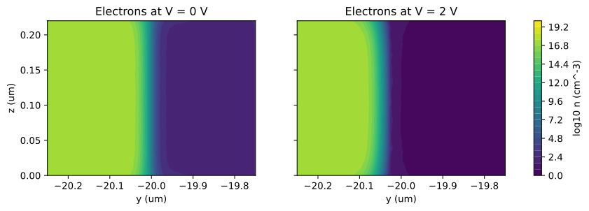
The electron concentration across the rib at the two ends of the sweep, on a log scale. The n side is on the left (high \(n\)), the p side on the right (almost no electrons), and the transition between them is the depletion edge. At 2 V it has moved further into the n side: that displacement, a few tens of nanometres, is the entire modulation mechanism.
A carrier map is sampled on the charge mesh nodes; its x_um is the in-plane
coordinate (device \(y\)) and its y_um the vertical one (device \(z\)).
fig, axes = plt.subplots(1, 2, figsize=(11, 3), sharey=True)
for ax, point in zip(axes, (sweep.points[0], sweep.points[-1]), strict=True):
    carriers = point.carriers
    tri = ax.tricontourf(
        carriers.x_um,
        carriers.y_um,
        np.log10(np.maximum(carriers.electrons_cm3, 1.0)),
        levels=30,
        rasterized=True,
    )
    ax.set_title(f"Electrons at V = {point.bias_v:g} V")
    ax.set_xlabel("y (um)")
    ax.set_xlim(*RIB_SPAN)
fig.colorbar(tri, ax=axes, label="log10 n (cm^-3)")
axes[0].set_ylabel("z (um)")
plt.show()
Step 2: from carriers to material properties
Free carriers change the silicon in two ways:
- At optical frequencies, the plasma-dispersion effect: an index change \(\Delta n\) (negative: carriers lower the index) and an absorption \(\Delta\alpha\). These are empirical power laws in \(n\) and \(p\); holes change the index more than electrons and absorb less for the same index change, which is why the junction is usually offset to put more of the mode on the p side.
- At RF, a conductivity \(\sigma = q(\mu_n n + \mu_p p)\): doped silicon is a (poor) conductor, a depleted region is an insulator. The mobilities \(\mu\) fall with doping, because carriers scatter off the dopant atoms: the contact regions are doped 300 times more heavily than the core but conduct only about 40 times better (compare the strip conductivities printed in Step 4).
carrier_response below is the one place where carriers become material
properties; both the optical and the RF steps call it. The optical coefficients
are the published silicon fits of Nedeljkovic et al. (2011) at 1.55 µm
(PlasmaDispersionModel.nedeljkovic_1310() is the 1.31 µm set;
foundry-calibrated values go in the same way). The mobility model is the
published silicon fit of Masetti et al. (1983), the one the charge solve uses
by default, so that both steps agree on the resistance of the silicon.
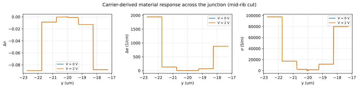
The plots are a horizontal cut through the middle of the rib. At the centre, where the silicon is depleted, all three quantities drop to zero, and that region is wider at 2 V.
from types import SimpleNamespace

from gsim.common.carriers import (
    MobilityModel,
    PlasmaDispersionModel,
    carrier_absorption_cm,
    carrier_conductivity,
    carrier_index_shift,
)

DISPERSION = PlasmaDispersionModel.nedeljkovic_1550()
MOBILITY = MobilityModel.masetti_silicon()


def carrier_response(n_cm3, p_cm3):
    """Index shift, absorption (1/cm) and conductivity (S/m) of carrier densities."""
    return SimpleNamespace(
        index_shift=carrier_index_shift(n_cm3, p_cm3, model=DISPERSION),
        absorption_cm=carrier_absorption_cm(n_cm3, p_cm3, model=DISPERSION),
        conductivity_s_per_m=carrier_conductivity(n_cm3, p_cm3, mobility=MOBILITY),
    )


fig, axes = plt.subplots(1, 3, figsize=(13, 3.2))
for point in (sweep.points[0], sweep.points[-1]):
    carriers = point.carriers
    cut = np.abs(carriers.y_um - RIB_HEIGHT / 2) < 0.03
    order = np.argsort(carriers.x_um[cut])
    response = carrier_response(
        carriers.electrons_cm3[cut][order], carriers.holes_cm3[cut][order]
    )
    y = carriers.x_um[cut][order]
    label = f"V = {point.bias_v:g} V"
    axes[0].plot(y, response.index_shift, label=label)
    axes[1].plot(y, response.absorption_cm, label=label)
    axes[2].plot(y, response.conductivity_s_per_m, label=label)
axes[0].set_ylabel("$\\Delta n$")
axes[1].set_ylabel("$\\Delta\\alpha$ (1/cm)")
axes[2].set_ylabel("$\\sigma$ (S/m)")
for ax in axes:
    ax.set_xlabel("y (um)")
    ax.grid(alpha=0.3)
    ax.legend(fontsize=8)
fig.suptitle("Carrier-derived material response across the junction (mid-rib cut)")
plt.tight_layout()
plt.show()
Step 3: the optical mode at each bias
The optical step meshes its own window around the rib with the same native-2D
mesher Palace uses (BoundaryModeSim, used here only to mesh), carries each
bias point's carrier map onto that mesh element by element
(transfer_carriers), and solves for the guided mode with femwell. Each element
of doped silicon takes \(\varepsilon = (n_{Si} + \Delta n - i\kappa)^2\), with
\(\kappa\) from the local absorption; every other element keeps its material's
permittivity. One complex effective index comes out per bias:
- the change of its real part with bias, \(\Delta n_{eff}(V)\), is the phase modulation;
- its imaginary part is the optical loss caused by the free carriers.
The window wall is a perfect conductor, and the carrier map is carried onto a mesh held to the same 10 nm across the rib as the charge mesh: a coarser one would smear the depletion edge again. The mesh does not move with the bias, only the permittivity of its elements, so it is built once.
from gsim.common.carrier_transfer import transfer_carriers
from gsim.common.carriers import permittivity_perturbation
from gsim.common.modes import select_line_mode
from gsim.femwell import boundary_field_ratio, epsilon_by_region, solve_modes
from gsim.palace import BoundaryModeSim


def cross_section_mesh(
    component, stack, *, plane, output_dir, window=None, window_z=None, boxes=None
):
    """Mesh a cross-section of a component in oxide and return the mesh path."""
    sim = BoundaryModeSim()
    sim.set_output_dir(output_dir)
    sim.set_stack(stack)
    sim.set_geometry(component)
    sim.set_airbox(
        margin_x=2.0, margin_y=2.0, z_above=1.5, z_below=1.0, material="sio2"
    )
    sim.set_cross_section(plane, window=window, window_z=window_z)
    sim.mesh(
        preset="coarse",
        refined_mesh_size=0.05,
        max_mesh_size=40.0,
        refinement_boxes=boxes,
        verbose=False,
    )
    return sim.mesh_path


optical_mesh = cross_section_mesh(
    component,
    stack,
    plane="x=0",
    output_dir="./tcad-twmzm/optical",
    window=OPTICAL_WINDOW,
    window_z=OPTICAL_WINDOW_Z,
    boxes=[JUNCTION_BOX],
)


def solve_optical_mode(carriers, wavelength_um=WAVELENGTH_UM):
    """Complex n_eff of the guided mode with one carrier map on the optical mesh."""
    base = epsilon_by_region(optical_mesh, stack, wavelength_um=wavelength_um)
    doped = [name for name in REGIONS if name in base]
    on_mesh = transfer_carriers(
        carriers, optical_mesh, at="elements", fill=0.0, regions=doped
    )
    response = carrier_response(on_mesh.electrons_cm3, on_mesh.holes_cm3)
    epsilon = np.array([base[name] for name in on_mesh.region], dtype=complex)
    for i, name in enumerate(on_mesh.region):
        if name in doped:
            epsilon[i] = permittivity_perturbation(
                n0=np.sqrt(base[name].real),
                dn=response.index_shift[i],
                dalpha_cm=response.absorption_cm[i],
                wavelength_um=wavelength_um,
            )
    modes = solve_modes(
        optical_mesh,
        epsilon=epsilon,
        wavelength_um=wavelength_um,
        metallic_boundaries=True,
    )
    mode = select_line_mode(modes)
    assert boundary_field_ratio(mode) < 0.01, "the optical window clips the mode"
    return complex(mode.n_eff)
n_eff = np.array([solve_optical_mode(point.carriers) for point in sweep.points])
index_shift = n_eff.real - n_eff[0].real
# |Im n_eff| is an amplitude decay: 4 pi |Im n_eff| / lambda per unit length in power.
loss_db_cm = 40 * np.pi / np.log(10) * np.abs(n_eff.imag) / (WAVELENGTH_UM * 1e-4)

for v, n, dn, loss in zip(sweep.voltages, n_eff, index_shift, loss_db_cm, strict=True):
    print(
        f"V = {v:4.1f} V:  n_eff = {n.real:.6f},  "
        f"dn_eff = {dn:+.2e},  loss = {loss:5.2f} dB/cm"
    )
V =  0.0 V:  n_eff = 2.568453,  dn_eff = +0.00e+00,  loss =  8.27 dB/cm
V =  0.2 V:  n_eff = 2.568466,  dn_eff = +1.25e-05,  loss =  8.05 dB/cm
V =  0.4 V:  n_eff = 2.568477,  dn_eff = +2.38e-05,  loss =  7.84 dB/cm
V =  0.6 V:  n_eff = 2.568488,  dn_eff = +3.42e-05,  loss =  7.65 dB/cm
V =  0.8 V:  n_eff = 2.568497,  dn_eff = +4.39e-05,  loss =  7.47 dB/cm
V =  1.0 V:  n_eff = 2.568506,  dn_eff = +5.30e-05,  loss =  7.31 dB/cm
V =  1.2 V:  n_eff = 2.568515,  dn_eff = +6.16e-05,  loss =  7.15 dB/cm
V =  1.4 V:  n_eff = 2.568523,  dn_eff = +6.98e-05,  loss =  7.00 dB/cm
V =  1.6 V:  n_eff = 2.568531,  dn_eff = +7.77e-05,  loss =  6.86 dB/cm
V =  1.8 V:  n_eff = 2.568539,  dn_eff = +8.52e-05,  loss =  6.73 dB/cm
V =  2.0 V:  n_eff = 2.568546,  dn_eff = +9.24e-05,  loss =  6.60 dB/cm
As the bias rises, carriers leave the centre of the mode: \(n_{eff}\) goes up and the loss goes down. Note the scale: the index moves in the fifth decimal place, which is why the mode solve needs the carrier map resolved rather than averaged.
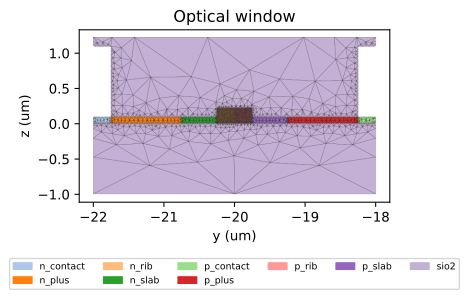
The optical mesh, for comparison with the charge mesh above: a smaller window, with the 10 nm elements across the rib and coarser ones around it, since away from the junction it resolves a wavelength-scale mode rather than a nanometre-scale depletion edge. The corner of the cathode metal reaching into the window is a hole in it.
fig, ax = plt.subplots(figsize=(8, 3.5))
plot_cross_section(optical_mesh, ax=ax, title="Optical window")
plt.tight_layout()
plt.show()
Modulation efficiency \(V_\pi L\) and optical loss
A phase shift of \(\pi\) over a length \(L\) needs \(\Delta n_{eff} = \lambda / 2L\), so the efficiency follows from the local slope of the curve on the left:
\(V_\pi L\) rises with bias because the depletion width grows like \(\sqrt{V}\): each extra volt moves the edge a little less than the previous one. The value is quoted one point before the end of the sweep, where the slope is a centred difference: 2.11 V·cm at 1.8 V, typical for this kind of junction.
There is a trade-off here. Heavier core doping improves \(V_\pi L\) and worsens the loss; the product of the two is the usual figure of merit when comparing junction designs.
from gsim.common.twmzm import vpi_length_vcm

vpi_l = vpi_length_vcm(sweep.voltages, index_shift, wavelength_um=WAVELENGTH_UM)

fig, axes = plt.subplots(1, 3, figsize=(13, 3.2))
axes[0].plot(sweep.voltages, index_shift * 1e5, "o-")
axes[0].set_ylabel("$\\Delta n_{eff} \\times 10^{5}$")
axes[1].plot(sweep.voltages, vpi_l, "o-")
axes[1].set_ylabel("$V_\\pi L$ (V cm)")
axes[2].plot(sweep.voltages, loss_db_cm, "o-")
axes[2].set_ylabel("optical loss (dB/cm)")
for ax in axes:
    ax.set_xlabel("Reverse bias (V)")
    ax.grid(alpha=0.3)
plt.tight_layout()
plt.show()
print(f"V_pi L at {sweep.voltages[-2]:.1f} V: {vpi_l[-2]:.2f} V cm")
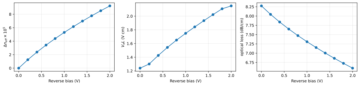
V_pi L at 1.8 V: 2.11 V cm
Step 4: the RF transmission line
Now the electrical side. Two electrodes, one on each contact region, form a transmission line, and the doped silicon between them loads it: the junction adds capacitance, and the resistive silicon on either side of it adds loss. This step finds the propagating mode of that loaded line and reads off its per-unit-length behaviour.
The staircase cross-section
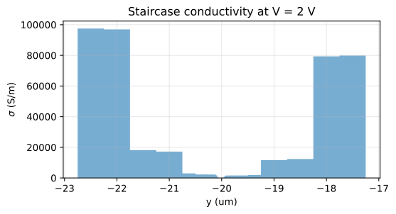
femwell accepts a continuous permittivity, but the line's current has to be read off well-defined conductors, and a Palace solve of the same line would take one constant material per region. So the RF cross-section is a staircase: the carrier map at one bias (the last of the sweep, 2 V) is cut into vertical strips, each with the conductivity of its average carrier concentrations.
The strips follow the drawn device: none straddles two doped regions, and each
has its own region's height (220 nm in the rib, 90 nm in the slab). The rib,
where the conductivity changes quickly, gets 21 strips; each of the other
regions gets two. Two 10 µm wide, 1 µm thick aluminium electrodes flank the
strips, as wide as a real traveling-wave line's, since the drawn component only
carries the metal where it lands. build_staircase_cross_section draws all of
it on a component of its own, with carrier_response turning each strip's
carriers into its conductivity.
The plot shows the result: highly conducting contact regions at both ends, then the plus regions, the lightly doped core, and at the centre a few strips with essentially zero conductivity. That insulating gap is the junction capacitor; the conducting silicon on each side is its series resistance.
from gsim.common.staircase import (
    ElectrodeSpec,
    RFStripMaterial,
    StaircaseDrawing,
    StripSegment,
    build_staircase_cross_section,
)

RF_BIAS = sweep.points[-1]
segments = [
    StripSegment(span=spans[name], z=(0.0, height), n_strips=2)
    for name, (_, _, height, _) in REGIONS.items()
    if name not in ("n_rib", "p_rib")
]
segments.append(StripSegment(span=RIB_SPAN, z=(0.0, RIB_HEIGHT), n_strips=21))
staircase = build_staircase_cross_section(
    RF_BIAS.carriers,
    segments=sorted(segments, key=lambda segment: segment.span),
    response=carrier_response,
    material=RFStripMaterial(permittivity=11.9, fmax_hz=max(RF_FREQS_HZ)),
    electrodes=ElectrodeSpec(width_um=10.0, thickness_um=METAL_THICKNESS),
    drawing=StaircaseDrawing(substrate_thickness=2.0),
)

edges = staircase.strips.edges_um
sigma = staircase.strips.conductivity_s_per_m
print("strip edges (um):", np.round(edges, 3))
print("strip sigma (S/m):", np.round(sigma, 1))
print(
    "electrodes (um):",
    dict(zip(staircase.electrode_names, staircase.electrode_spans, strict=True)),
)

fig, ax = plt.subplots(figsize=(6, 3))
ax.stairs(sigma, edges, fill=True, alpha=0.6)
ax.set_xlabel("y (um)")
ax.set_ylabel("$\\sigma$ (S/m)")
ax.set_title(f"Staircase conductivity at V = {RF_BIAS.bias_v:g} V")
ax.grid(alpha=0.3)
plt.show()
strip edges (um): [-22.75  -22.25  -21.75  -21.25  -20.75  -20.5   -20.25  -20.226 -20.202
 -20.179 -20.155 -20.131 -20.107 -20.083 -20.06  -20.036 -20.012 -19.988
 -19.964 -19.94  -19.917 -19.893 -19.869 -19.845 -19.821 -19.798 -19.774
 -19.75  -19.5   -19.25  -18.75  -18.25  -17.75  -17.25 ]
strip sigma (S/m): [9.75194e+04 9.69603e+04 1.81474e+04 1.72039e+04 3.00050e+03 2.28690e+03
 2.22780e+03 2.26960e+03 2.26800e+03 2.25950e+03 2.23930e+03 2.17150e+03
 1.71170e+03 3.69900e+02 5.00000e-01 0.00000e+00 0.00000e+00 5.20000e+00
 7.18100e+02 1.50370e+03 1.59890e+03 1.61380e+03 1.62050e+03 1.62410e+03
 1.62730e+03 1.62820e+03 1.60660e+03 1.63360e+03 1.98330e+03 1.16431e+04
 1.23573e+04 7.93550e+04 7.98879e+04]
electrodes (um): {'electrode_low': (-32.75, -22.75), 'electrode_high': (-17.25, -7.25)}
Line parameters versus frequency
The staircase is meshed once, then the line mode is solved at each frequency, with every material resolved there: the strips' and the aluminium's conductivity become an imaginary permittivity \(-\sigma/\omega\varepsilon_0\). Three numbers come out per frequency:
- the RF index \(n_{RF}\): how slowly the RF wave travels (\(v = c/n_{RF}\));
- the RF loss \(\alpha_{RF}\) in dB/cm;
- the characteristic impedance \(Z_0 = 2P/|I|^2\), from the power carried by the mode and the current in the signal electrode, the one on the cathode.
These come directly from the field solution; no analytic transmission-line
formula is involved. Four modes are solved per frequency and the slowest
propagating one is the line mode (select_line_mode); each frequency's
eigenvalue search is aimed at the index solved at the one before, so the sweep
stays on the same mode. line_reading also compares the two electrode currents,
which tells the line mode, with opposite currents, from a mode returning its
current through the window wall.
from scipy.constants import speed_of_light

from gsim.common.transmission_line import line_params_from_neff
from gsim.femwell import line_reading

rf_mesh = cross_section_mesh(
    staircase.component,
    staircase.stack(),
    plane="x=5",  # the middle of the staircase's 10 um drawn length
    output_dir="./tcad-twmzm/rf",
)
signal = staircase.conductor("electrode_low")  # on the cathode side
ground = staircase.conductor("electrode_high")

rf_n_eff, rf_z0, guess = [], [], 3.0
for freq in RF_FREQS_HZ:
    modes = solve_modes(
        rf_mesh,
        epsilon=epsilon_by_region(rf_mesh, staircase.stack(), frequency_hz=freq),
        wavelength_um=speed_of_light / freq * 1e6,
        num_modes=4,
        metallic_boundaries=True,
        n_guess=guess,
    )
    reading = line_reading(
        select_line_mode(modes),
        frequency_hz=freq,
        mesh=rf_mesh,
        signal=signal,
        return_=ground,
    )
    assert not reading.wall_mode, reading.diagnostic
    rf_n_eff.append(reading.n_eff)
    rf_z0.append(reading.z0_ohm)
    guess = reading.n_eff.real

line_params = line_params_from_neff(
    RF_FREQS_HZ, rf_n_eff, z0_ohm=rf_z0, bias_v=RF_BIAS.bias_v
)
for freq, n_rf, alpha, z0 in zip(
    line_params.freq_hz,
    line_params.n_rf,
    line_params.alpha_rf_np_m,
    line_params.z0_ohm,
    strict=True,
):
    print(
        f"f = {freq / 1e9:5.0f} GHz:  n_RF = {n_rf:5.2f},  "
        f"alpha_RF = {alpha * 8.686 / 100:5.1f} dB/cm,  Z0 = {z0.real:5.1f} ohm"
    )
f =     1 GHz:  n_RF =  5.55,  alpha_RF =   7.8 dB/cm,  Z0 =  34.2 ohm
f =     2 GHz:  n_RF =  4.66,  alpha_RF =   9.4 dB/cm,  Z0 =  29.3 ohm
f =     5 GHz:  n_RF =  4.11,  alpha_RF =  12.5 dB/cm,  Z0 =  27.1 ohm
f =    10 GHz:  n_RF =  3.86,  alpha_RF =  17.3 dB/cm,  Z0 =  26.9 ohm
f =    20 GHz:  n_RF =  3.66,  alpha_RF =  29.0 dB/cm,  Z0 =  27.1 ohm
f =    40 GHz:  n_RF =  3.37,  alpha_RF =  60.7 dB/cm,  Z0 =  28.1 ohm
f =    60 GHz:  n_RF =  3.12,  alpha_RF =  93.2 dB/cm,  Z0 =  29.6 ohm
f =    80 GHz:  n_RF =  2.91,  alpha_RF = 120.5 dB/cm,  Z0 =  31.1 ohm
f =   100 GHz:  n_RF =  2.77,  alpha_RF = 141.9 dB/cm,  Z0 =  32.6 ohm
Three things to read from this table:
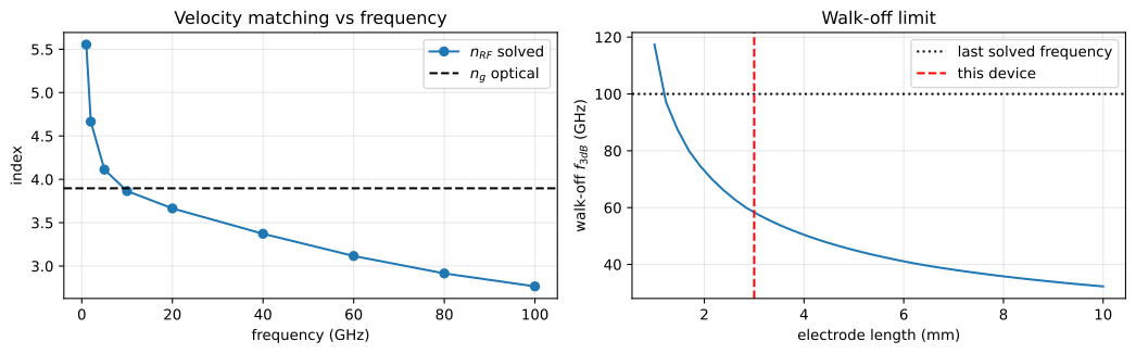
- \(n_{RF}\) falls from 5.62 at 1 GHz to 2.76 at 100 GHz, where a line in oxide alone would sit near \(\sqrt{\varepsilon_{SiO_2}} \approx 2\). The junction capacitance slows the wave down, a slow-wave line, which is what brings the RF velocity close to the optical one (\(n_g \approx 3.89\), computed in Step 5). The slowing fades at high frequency, where the junction capacitor no longer has time to charge through the resistive silicon.
- \(Z_0\) stays between 26.1 and 33.3 Ω, for the same reason: extra capacitance per unit length lowers the impedance. Real designs space the electrodes further apart, or load the line only periodically, to get closer to 50 Ω.
- The RF loss grows quickly with frequency. The current that charges the junction capacitor flows through resistive silicon, and that charging current grows with frequency. This demonstration device is not optimised and is heavily loaded.
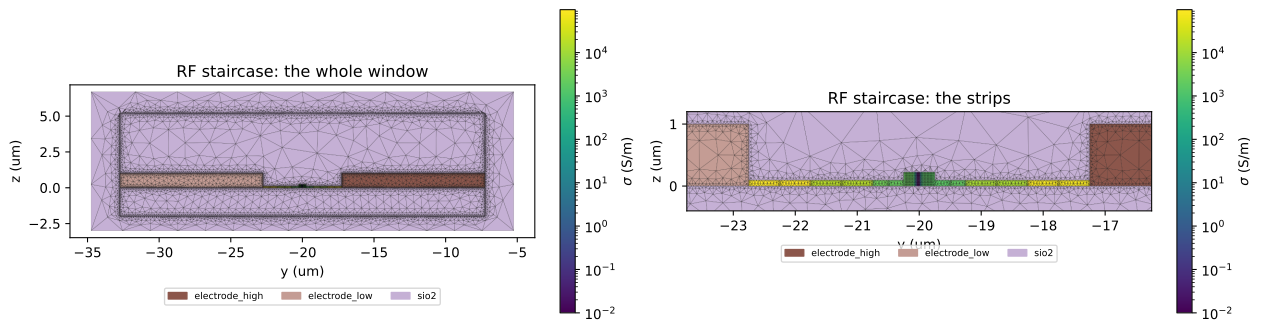
Below is the mesh the line was solved on: the strips coloured by conductivity, between the two electrodes, in oxide. In the close-up the depleted strips at the junction are the dark band at the centre.
strip_sigma = dict(zip(staircase.strip_names, sigma, strict=True))
fig, axes = plt.subplots(1, 2, figsize=(13, 4))
for ax, title, xlim, ylim in (
    (axes[0], "RF staircase: the whole window", None, None),
    (
        axes[1],
        "RF staircase: the strips",
        (edges[0] - 1.0, edges[-1] + 1.0),
        (-0.4, 1.2),
    ),
):
    plot_cross_section(
        rf_mesh,
        ax=ax,
        title=title,
        values=strip_sigma,
        label="$\\sigma$ (S/m)",
        xlim=xlim,
        ylim=ylim,
    )
plt.tight_layout()
plt.show()
Step 5: the whole device
Velocity mismatch
The light travels at the optical group velocity (\(c/n_g\)), the RF wave at \(c/n_{RF}\). If the two differ, the light gradually slips relative to the RF wave and, over a long enough electrode, sees the drive voltage average out. For a lossless, matched line this alone limits the bandwidth to
so a longer modulator (lower drive voltage) has a lower walk-off limit.
A single-wavelength mode solve gives the phase index, not the group index, so the optical mode is solved again 10 nm either side of the wavelength, at 0 V, with every material re-resolved there, and \(n_g = n_{eff} - \lambda\, dn_{eff}/d\lambda\).
On a loaded line \(n_{RF}\) falls with frequency, so the mismatch in the formula
is the one the line has at the frequency in question:
walkoff_bandwidth_dispersive solves for the frequency that satisfies the
condition with its own \(n_{RF}(f)\). Beyond the last solved frequency it keeps
the last solved index, so values above the dotted line in the right-hand plot
are extrapolations.
On this device \(n_{RF}\) starts well above \(n_g\) (by 1.73 at 1 GHz), crosses it near 10 GHz and ends well below it (by 1.13 at 100 GHz). The walk-off limit for the 3 mm electrode, 58.4 GHz in the next section's printout, is about six times the electro-optic bandwidth, so velocity mismatch is not what limits this modulator.
STEP_UM = 0.01
n_below, n_above = (
    solve_optical_mode(sweep.points[0].carriers, WAVELENGTH_UM + step).real
    for step in (-STEP_UM, STEP_UM)
)
N_GROUP = n_eff[0].real - WAVELENGTH_UM * (n_above - n_below) / (2 * STEP_UM)
print(f"n_eff = {n_eff[0].real:.4f}, n_g = {N_GROUP:.4f}")
print(
    f"  from n_eff = {n_below:.4f} / {n_above:.4f} at "
    f"{WAVELENGTH_UM - STEP_UM:g} / {WAVELENGTH_UM + STEP_UM:g} um"
)
n_eff = 2.5685, n_g = 3.8968
  from n_eff = 2.5770 / 2.5599 at 1.54 / 1.56 um
from gsim.common.twmzm import walkoff_bandwidth_dispersive

lengths_mm = np.linspace(1, 10, 40)
walkoff_ghz = [
    (
        walkoff_bandwidth_dispersive(
            line_params.freq_hz, line_params.n_rf, length_m=length * 1e-3, n_opt=N_GROUP
        )
        or np.nan
    )
    / 1e9
    for length in lengths_mm
]

fig, axes = plt.subplots(1, 2, figsize=(11, 3.5))
axes[0].plot(line_params.freq_hz / 1e9, line_params.n_rf, "o-", label="$n_{RF}$ solved")
axes[0].axhline(N_GROUP, color="k", ls="--", label="$n_g$ optical")
axes[0].set_xlabel("frequency (GHz)")
axes[0].set_ylabel("index")
axes[0].set_title("Velocity matching vs frequency")
axes[0].legend()
axes[1].plot(lengths_mm, walkoff_ghz)
axes[1].axhline(
    max(RF_FREQS_HZ) / 1e9, color="k", ls=":", label="last solved frequency"
)
axes[1].axvline(LENGTH_UM * 1e-3, color="r", ls="--", label="this device")
axes[1].set_xlabel("electrode length (mm)")
axes[1].set_ylabel("walk-off $f_{3dB}$ (GHz)")
axes[1].set_title("Walk-off limit")
axes[1].legend()
for ax in axes:
    ax.grid(alpha=0.3)
plt.tight_layout()
plt.show()
Electro-optic response and figures of merit
The cross-section does not know three things about the device: the electrode
length, the source impedance driving it and the termination at its
end. twmzm_figures_of_merit adds them and computes the standard small-signal
traveling-wave response: the RF voltage wave along the line, including
attenuation and the reflections at both ends, averaged over the transit of the
light. Velocity mismatch, RF loss and impedance mismatch are all included. It
takes the RF line parameters and the optical bias sweep (OpticalPhaseSweep:
index shift and loss versus bias, and the group index).
Here the line is driven from 50 Ω and terminated in its own characteristic impedance, so nothing reflects from the far end. The response is evaluated on a finer frequency grid than the line was solved on, by interpolation within the solved range, so the 3 dB point can be read accurately.
from gsim.common.twmzm_report import OpticalPhaseSweep, twmzm_figures_of_merit

optical_sweep = OpticalPhaseSweep(
    voltages_v=sweep.voltages,
    dn_eff=index_shift,
    alpha_opt_db_cm=loss_db_cm,
    wavelength_um=WAVELENGTH_UM,
    n_group=N_GROUP,
)
# A denser grid than the line was solved on, kept inside the solved range.
response_grid = line_params.resampled(
    np.linspace(min(RF_FREQS_HZ), max(RF_FREQS_HZ), 200)
)
Z_LOAD = float(np.mean(line_params.z0_ohm.real))  # terminate in the line


def device_report(length_um, **mach_zehnder):
    """Figures of merit of an electrode of this length, 50 ohm source, matched load."""
    return twmzm_figures_of_merit(
        response_grid,
        optical_sweep,
        length_m=length_um * 1e-6,
        z_load_ohm=Z_LOAD,
        z_gen_ohm=50.0,
        **mach_zehnder,
    )


report = device_report(LENGTH_UM)

fig, ax = plt.subplots(figsize=(7, 4))
ax.plot(report.freq_hz / 1e9, 20 * np.log10(np.abs(report.response)))
ax.axhline(20 * np.log10(1 / np.sqrt(2)), color="k", ls=":", label="-3 dB (EO)")
if report.bandwidth_3db_hz:
    ax.axvline(report.bandwidth_3db_hz / 1e9, color="r", ls="--")
ax.set_xlabel("frequency (GHz)")
ax.set_ylabel("EO response (dB)")
ax.set_title(f"TW-MZM response, L = {report.length_m * 1e3:.0f} mm, matched load")
ax.legend()
ax.grid(alpha=0.3)
plt.show()

print("=== TW-MZM figures of merit ===")
if report.bandwidth_3db_hz:
    print(f"EO 3 dB bandwidth:        {report.bandwidth_3db_hz / 1e9:.1f} GHz")
elif report.bandwidth_message:
    print(f"EO 3 dB bandwidth:        {report.bandwidth_message}")
if report.walkoff_bandwidth_hz:
    print(f"walk-off limit:           {report.walkoff_bandwidth_hz / 1e9:.1f} GHz")
print(
    f"velocity mismatch:        n_RF - n_g = {report.velocity_mismatch[0]:+.2f} at "
    f"{report.freq_hz[0] / 1e9:.0f} GHz, {report.velocity_mismatch[-1]:+.2f} at "
    f"{report.freq_hz[-1] / 1e9:.0f} GHz"
)
print(f"characteristic impedance: {report.z0_ohm[0].real:.1f} ohm")
print(
    f"V_pi L at {report.voltages_v[-2]:.1f} V:        {report.vpi_l_vcm[-2]:.2f} V cm"
)
rlgc = report.rlgc
print(
    f"RLGC at 10 GHz: R = {np.interp(10e9, report.freq_hz, rlgc['R']):.0f} ohm/m, "
    f"L = {np.interp(10e9, report.freq_hz, rlgc['L']) * 1e9:.0f} nH/m, "
    f"C = {np.interp(10e9, report.freq_hz, rlgc['C']) * 1e12:.0f} pF/m"
)
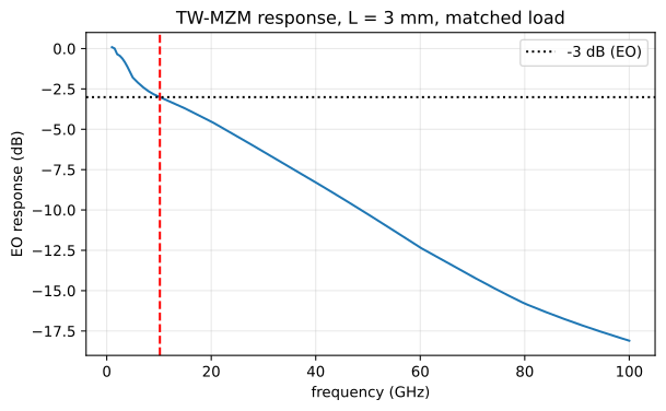
=== TW-MZM figures of merit ===
EO 3 dB bandwidth:        10.2 GHz
walk-off limit:           58.3 GHz
velocity mismatch:        n_RF - n_g = +1.66 at 1 GHz, -1.13 at 100 GHz
characteristic impedance: 34.2 ohm
V_pi L at 1.8 V:        2.11 V cm
RLGC at 10 GHz: R = 6353 ohm/m, L = 343 nH/m, C = 483 pF/m
The electro-optic bandwidth is 9.7 GHz, about a sixth of the 58.4 GHz walk-off limit: this device is limited by RF loss, already 7.9 dB/cm at 1 GHz and 17.6 dB/cm at 10 GHz. The response is normalised to DC, below the first solved frequency: there the reverse-biased junction draws no current and the line is taken as lossless, a reference the solved loss falls towards (12.7 dB/cm at 5 GHz, 7.9 dB/cm at 1 GHz). Starting the sweep at 1 GHz resolves the roll-off between there and the 3 dB point. The way to improve it is to reduce the series resistance of the silicon or the loading of the line, not to tune the velocity match.
The report also gives the line's RLGC parameters (series resistance and inductance, shunt conductance and capacitance per unit length), derived from \(\gamma\) and \(Z_0\). They are what a circuit simulator needs.
From phase shifter to modulator: transfer, \(V_\pi\), extinction and chirp
So far the report describes the phase shifter. A modulator puts one in each arm of a Mach-Zehnder interferometer, and what you measure on the bench is the optical power out against the drive voltage. The same report computes that static transfer \(T(v)\) from the optical bias sweep (index shift and loss versus bias) and the electrode length, and reads the datasheet numbers off it:
- \(V_\pi\): the drive swing from the peak of the transfer to the adjacent null, at this length (not the length-independent \(V_\pi L\) above);
- insertion loss: the transmission at the peak;
- extinction ratio: peak over null. It is finite because the two arms sit at
different voltages at the null, so their free-carrier losses differ and the
fields do not cancel, and because a real splitter is never exactly 50:50
(
arm_imbalance_db); - chirp: the small-signal chirp parameter at each bias point, from the index and absorption slopes. Positive means the optical frequency rises while the intensity rises.
The drive voltage \(v\) is the voltage between the two arms. "single-drive" puts
all of it on one arm and leaves the other at the arm bias; "push-pull" moves
the arms by \(\pm v/2\) about it. Both arms rest in the middle of the bias sweep
unless you set arm_bias_v, and the interferometer is parked at quadrature
(phase_offset_rad), where it rests at half its peak transmission. Nothing is
extrapolated: the transfer only covers the drive the bias sweep can answer for,
which is twice as wide for push-pull. If the sweep is too short to go from a
peak to a null, \(V_\pi\), insertion loss and extinction ratio are left out and
transfer_message says why; sweep more bias or lengthen the electrode. None of
this re-runs a solver.
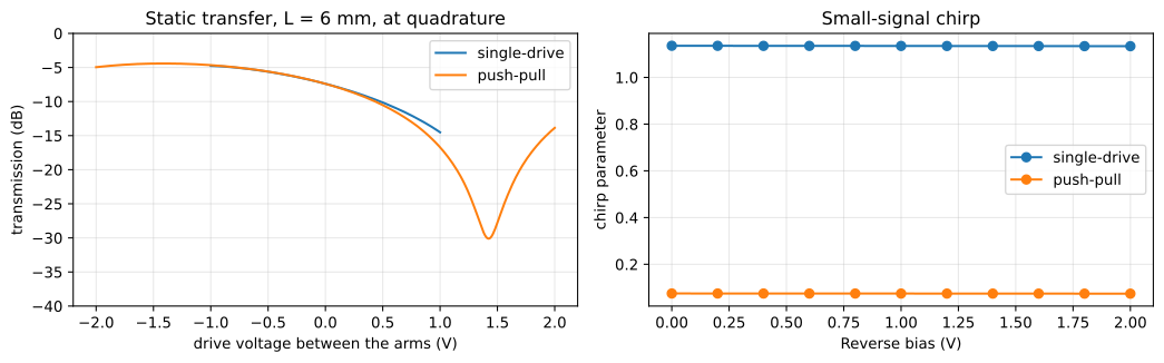
That last point bites here: with \(V_\pi L\) near 2.1 V·cm, the 3 mm electrode has a \(V_\pi\) close to 7 V, and the 0 to 2 V bias sweep cannot swing either configuration from a peak to a null. So this section looks at a 6 mm electrode, the length at which a push-pull drive fits inside the sweep, with a 0.2 dB splitter imbalance; the rest of the notebook stays at 3 mm.
MZ_LENGTH_UM = 6000.0  # long enough for a push-pull V_pi inside the 0-2 V sweep

mz_reports = {
    drive: device_report(MZ_LENGTH_UM, drive=drive, arm_imbalance_db=0.2)
    for drive in ("single-drive", "push-pull")
}

fig, axes = plt.subplots(1, 2, figsize=(11, 3.5))
for drive, rep in mz_reports.items():
    axes[0].plot(rep.drive_v, 10 * np.log10(rep.transfer), label=drive)
    axes[1].plot(rep.voltages_v, rep.chirp, "o-", label=drive)
axes[0].set_xlabel("drive voltage between the arms (V)")
axes[0].set_ylabel("transmission (dB)")
axes[0].set_ylim(-40, 0)
axes[0].set_title(f"Static transfer, L = {MZ_LENGTH_UM * 1e-3:.0f} mm, at quadrature")
axes[1].set_xlabel("Reverse bias (V)")
axes[1].set_ylabel("chirp parameter")
axes[1].set_title("Small-signal chirp")
for ax in axes:
    ax.legend()
    ax.grid(alpha=0.3)
plt.tight_layout()
plt.show()

for drive, rep in mz_reports.items():
    print(f"=== {drive} (arms resting at {rep.arm_bias_v:.1f} V) ===")
    if rep.v_pi_v is None:
        print(rep.transfer_message)
    else:
        print(f"V_pi:              {rep.v_pi_v:.2f} V")
        print(f"insertion loss:    {rep.insertion_loss_db:.1f} dB")
        print(f"extinction ratio:  {rep.extinction_ratio_db:.1f} dB")
    print(
        f"chirp:             {rep.chirp[0]:+.2f} to {rep.chirp[-1]:+.2f} along the sweep"
    )
=== single-drive (arms resting at 1.0 V) ===
The bias sweep is too short to reach V_pi: its single-drive span of -1 to 1 V moves the arm phase difference by 0.72 pi and does not take the transfer from a peak to a null, so V_pi, the insertion loss and the extinction ratio are not reported rather than extrapolated. Widen the bias sweep or lengthen the electrode.
chirp:             +1.14 to +1.13 along the sweep
=== push-pull (arms resting at 1.0 V) ===
V_pi:              2.86 V
insertion loss:    4.4 dB
extinction ratio:  25.7 dB
chirp:             +0.07 to +0.07 along the sweep
Single-drive chirp sits near \(+1\) (+1.14) at this quadrature point; the other
one, phase_offset_rad=-np.pi/2, makes it negative. Push-pull cancels it down to
+0.07, the small residue left by the two arms' losses moving in opposite
directions and by the splitter imbalance. Push-pull also reaches \(V_\pi\) from a
bias sweep half as wide: at 6 mm it swings from peak to null in 2.86 V, with
4.4 dB insertion loss and 25.7 dB extinction, while the single drive prints the
"too short" message, its sweep moving the arm phase difference by only
0.71 π at this length.
Summary
Starting from one gdsfactory component and one layer stack, and calling the gsim building blocks directly:
- DEVSIM (
gsim.tcad) solved the carrier distribution at each bias and the junction capacitance: the textbook formula for the depleted silicon, plus the 100 to 123 pF/m that fringes through the oxide around it; carrier_responseconverted those maps into an optical index change, an optical absorption and an RF conductivity;- femwell solved the optical mode on the continuous carrier profile, giving \(\Delta n_{eff}(V)\), the optical loss and \(V_\pi L\), and the RF mode of the loaded electrodes on a staircase, giving \(n_{RF}\), the RF loss and \(Z_0\);
twmzm_figures_of_meritcombined them into the electro-optic response, its 3 dB bandwidth, the RLGC parameters and the Mach-Zehnder transfer.
Things to try from here:
- your own device: replace the drawing cell with your component and stack, and name your doped regions, contacts and interfaces in Step 1;
- another wavelength:
WAVELENGTH_UM = 1.31withPlasmaDispersionModel.nedeljkovic_1310(); - a different junction: change the doping in
REGIONSand watch \(V_\pi L\) trade against loss; - a different electrode: change its geometry or
LENGTH_UM, and see \(Z_0\) and the bandwidth move.
Possible extensions of this flow: solving the same staircase with Palace
(BoundaryModeSim.run_local), cross-checking the loaded line against the bare
electrode plus a lumped junction branch (sweep.junction_branch()), comparing a
graded junction (tcad.TableDoping), and segmenting the electrode toward 50 Ω
(gsim.common.transmission_line.segmented_line).