Terminal (multi-pin) wave ports in Palace
A wave port reports modal S-parameters. A circuit needs terminal S-parameters: one port per conductor, with a reference impedance you choose. This notebook builds the terminal S-parameters of a coupled GSSG line on the generic PDK, following the guide Terminal (multi-pin) Wave Ports:
- a 2D
BoundaryModeSimon the port plane gives the terminal voltages and currents of every mode (T_V,T_I), with the conductors as perfect conductors like the port eigenproblem of the 3D run; - a 3D
DrivenSimwith one multimode wave port per end gives the modal S-parameters; terminal_spairs the 2D and 3D modes, putsT_VandT_Iinto the gauge of Palace's port modes and converts.
The notebook has two parts. Everything up to the cloud sections runs locally: geometry, terminal layout and voltage
paths, 2D and 3D meshing, the generated Palace configuration and the job sizes. The cloud sections are present but
guarded by RUN_CLOUD = False; they need a GDSFactory+ account and are run by hand.
Two lines are used, both on metal3 of the generic PDK (S width 10 um, gap 6 um, edge-to-edge S-S spacing 20 um,
G width 40 um, length 300 um, 1 to 50 GHz):
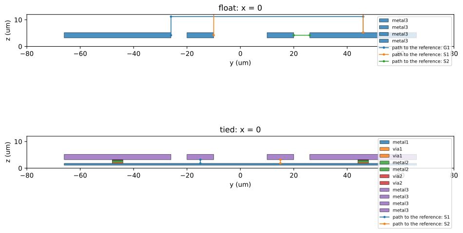
float: GSSG with floating outer grounds. Terminals G1, S1, S2, reference G2: three terminals, three modes.tied: the outer grounds tied by ametal1plane and continuous via walls. Terminals S1, S2, reference the plane: two terminals, two modes.
import json
import tempfile
from pathlib import Path

import gdsfactory as gf
import matplotlib.pyplot as plt
import numpy as np

import gsim
from gsim.common.cross_section import extract_plane_section
from gsim.common.modes import Conductor
from gsim.common.stack import get_stack
from gsim.palace import (
    BoundaryModeSim,
    DrivenSim,
    TerminalPortSpec,
    declare_terminal_paths,
    plot_plane_section,
    terminal_paths,
)
from gsim.palace.ports.modes import read_port_modes

gf.gpdk.PDK.activate()
LAYER = gf.gpdk.LAYER

# Submit the cloud jobs of sections 5 to 7 when True. Off: the notebook is a local dry run.
RUN_CLOUD = False
# The line to work on: "float" (three terminals) or "tied" (two terminals).
KIND = "float"

WORK = Path(tempfile.mkdtemp(prefix="palace-terminal-"))
1. Geometry
The four strips sit on metal3. The tied line adds a metal1 plane under the whole width and a 4 um wide wall of
via2, metal2 and via1 under each outer ground, so the two grounds and the plane are one conductor. The ports sit at
the signal centre (between the two signals); with max_size=True the port face is the whole simulation domain, so it
holds every conductor.
LENGTH = 300.0  # um
S_W, GAP, SS, G_W = (
    10.0,
    6.0,
    20.0,
    40.0,
)  # signal width, gap, edge-to-edge S-S spacing, ground width
WALL_W = 4.0  # width of the via walls under the outer grounds
FMIN, FMAX, NUM_POINTS = 1e9, 50e9, 50
# The 2D solves (section 3): gauge solves with PEC conductors, at the frequencies where 3D run 1 saves Palace's
# own port-mode fields, and lossy solves for the propagation constant gamma of the line.
FREQS_GAUGE = (1e9, 10e9, 50e9)
FREQS_LOSSY = (1e9, 5e9, 20e9, 50e9)
assert all(
    np.isclose(np.linspace(FMIN, FMAX, NUM_POINTS), f).any() for f in FREQS_GAUGE
)

S_IN = SS / 2
STRIPS = {  # (y0, y1) of every strip
    "G1": (-(S_IN + S_W + GAP + G_W), -(S_IN + S_W + GAP)),
    "S1": (-(S_IN + S_W), -S_IN),
    "S2": (S_IN, S_IN + S_W),
    "G2": (S_IN + S_W + GAP, S_IN + S_W + GAP + G_W),
}
Y_EDGE = STRIPS["G2"][1]

stack = get_stack()
Z = {
    name: (stack.layers[name].zmin, stack.layers[name].zmax)
    for name in ("metal1", "metal3")
}
MARGIN_Y, Z_ABOVE, Z_BELOW = 60.0, 60.0, 20.0  # airbox margins (um)
Z_OXIDE = (-2.0, 5.2)  # the oxide slab of set_stack(substrate_thickness=2.0)
# the meshed domain of every run below: the port face and the 2D cross-section
DOMAIN = (
    (-(Y_EDGE + MARGIN_Y), Y_EDGE + MARGIN_Y),
    (Z_OXIDE[0] - Z_BELOW, Z_OXIDE[1] + Z_ABOVE),
)


def _rect(c, y0, y1, layer):
    c.add_polygon(
        [(-LENGTH / 2, y0), (LENGTH / 2, y0), (LENGTH / 2, y1), (-LENGTH / 2, y1)],
        layer=layer,
    )


def build_component(kind):
    # The "float" or "tied" line with ports o1 (x < 0) and o2 (x > 0).
    c = gf.Component()
    for y0, y1 in STRIPS.values():
        _rect(c, y0, y1, LAYER.M3)
    if kind == "tied":
        _rect(c, -Y_EDGE, Y_EDGE, LAYER.M1)
        for name in ("G1", "G2"):
            y_mid = sum(STRIPS[name]) / 2
            for layer in (LAYER.VIA1, LAYER.M2, LAYER.VIA2):
                _rect(c, y_mid - WALL_W / 2, y_mid + WALL_W / 2, layer)
    for name, x, angle in (("o1", -LENGTH / 2, 180), ("o2", LENGTH / 2, 0)):
        c.add_port(
            name=name,
            center=(x, 0),
            width=S_W,
            orientation=angle,
            port_type="electrical",
            layer=LAYER.M3,
        )
    return c


def make_spec(kind, name="P"):
    # The terminals and the reference as rectangles (h = y, v = z, um) of the x = const cross-section.
    z3 = Z["metal3"]
    if kind == "float":
        terminals = [Conductor(n, (STRIPS[n], z3)) for n in ("G1", "S1", "S2")]
        reference = Conductor("G2", (STRIPS["G2"], z3))
    else:
        terminals = [Conductor(n, (STRIPS[n], z3)) for n in ("S1", "S2")]
        reference = Conductor("PLANE", ((-Y_EDGE, Y_EDGE), Z["metal1"]))
    return TerminalPortSpec(name=name, terminals=terminals, reference=reference)


NUM_MODES = {"float": 3, "tied": 2}
print(
    {k: len(make_spec(k).terminals) for k in NUM_MODES}, "terminals;", "domain", DOMAIN
)
{'float': 3, 'tied': 2} terminals; domain ((-126.0, 126.0), (-22.0, 65.2))
2. Terminal layout and voltage paths
terminal_paths draws one voltage path per terminal, from the terminal to the reference conductor. A path never crosses
a conductor: it goes straight across the gap when the terminal and the reference face each other, otherwise out of the
terminal at mid-height, over the metal and down onto the reference. The same paths are declared on the 2D solve (Palace
then writes the voltage of every mode on every path to mode-V.csv) and, for one pilot terminal per mode, on the 3D
port as its VoltagePath.
fig, axes = plt.subplots(2, 1, figsize=(10, 7))
for ax, kind in zip(axes, ("float", "tied"), strict=True):
    section = extract_plane_section(
        build_component(kind).copy(), stack, axis="x", value=0.0
    )
    plot_plane_section(
        section,
        h_range=(-80, 80),
        v_range=(0, 12),
        title=f"{kind}: x = 0",
        ax=ax,
        legend=False,
    )
    for name, points in terminal_paths(make_spec(kind), DOMAIN).items():
        h, v = zip(*points, strict=True)
        ax.plot(h, v, "-o", ms=2.5, lw=1.2, label=f"path to the reference: {name}")
    ax.legend(loc="upper right", fontsize=7)
plt.tight_layout()
plt.show()
3. The 2D solves (local meshing)
One BoundaryModeSim per frequency on the plane x = 0, with metallic_boundaries=True because the 3D port solve
treats the outer wall as PEC. The port solve also treats the finite-conductivity conductor surfaces as PEC, whereas a 2D
solve keeps them as Robin conductivity conditions unless conductor_boundary="pec" is set: its modes are then lossy, with
a complex, frequency-dependent n_eff (about 12 % away from the port solve's at 1 GHz on this line), and cannot be paired
with the port modes within 0.5 %. There are therefore two kinds of 2D solve:
- gauge solves (
conductors="pec"): the modes of the port eigenproblem. They giveT_V,T_Iand then_effthatalign_gaugepairs with the 3D port modes. With PEC conductors they hardly move with frequency, so a few solves are enough; they are at the frequencies where 3D run 1 saves Palace's own port-mode fields (FREQS_GAUGE). - lossy solves (
conductors="conductivity", the default ofBoundaryModeSim): the physical line. Only their propagation constantgamma = j k0 n_effis used, as the reference of the uniform-line check (FREQS_LOSSY).
The shielded domain has the outer wall as one more conductor, so one mode more than terminals is asked for and saved; the
extra mode is the wall mode, expected last by effective index (check mode-kn.csv after the run). The mode solve itself
needs Palace and runs in the cloud (section 5).
MESH_2D = {
    "preset": "default",
    "refined_mesh_size": 1.0,
    "max_mesh_size": 20.0,
    "fmax": FMAX,
}


def build_2d(kind, freq_hz, out, *, conductors="pec", target=0.0):
    # A configured, meshed BoundaryModeSim on x = 0 with the terminal paths declared.
    # conductors="pec": a gauge solve (the conductor surfaces are perfect conductors, as in the 3D port
    # eigenproblem); "conductivity": the lossy line, solved for its propagation constant only.
    gauge = conductors == "pec"
    sim = BoundaryModeSim()
    sim.set_output_dir(str(out))
    sim.set_geometry(build_component(kind))
    sim.set_stack(substrate_thickness=2.0)
    sim.set_airbox(margin_x=0.0, margin_y=MARGIN_Y, z_above=Z_ABOVE, z_below=Z_BELOW)
    sim.set_cross_section("x=0")
    sim.set_boundary_mode(
        freq=freq_hz,
        num_modes=NUM_MODES[kind] + 1,
        save=NUM_MODES[kind] + 1 if gauge else 0,
        target=target,
    )
    sim.metallic_boundaries = True
    sim.conductor_boundary = conductors
    sim.mesh(verbose=False, **MESH_2D)
    # Palace controls its path integration; mode-V.csv is a separate cross-check.
    indices = declare_terminal_paths(sim, make_spec(kind), sim.mesh_extent)
    return sim, indices


sim_2d, path_indices = build_2d(KIND, 20e9, WORK / "2d")
domain = sim_2d.mesh_extent
assert np.allclose(np.array(domain), np.array(DOMAIN)), (domain, DOMAIN)
print("2D domain (h, v):", domain)
print("palace path indices:", path_indices, [p.name for p in sim_2d.mode_paths])
print("validate_config:", sim_2d.validate_config().valid)

# What conductors="pec" changes: the conductor attributes move from Conductivity to PEC, nothing else.
sim_lossy, _ = build_2d(KIND, 20e9, WORK / "2d_lossy", conductors="conductivity")
boundaries = {
    name: json.loads(Path(s.write_config()).read_text())["Boundaries"]
    for name, s in (("gauge", sim_2d), ("lossy", sim_lossy))
}
robin = sorted(a for e in boundaries["lossy"]["Conductivity"] for a in e["Attributes"])
print(
    "lossy solve: Conductivity attributes",
    robin,
    "| PEC",
    boundaries["lossy"]["PEC"]["Attributes"],
)
print(
    "gauge solve: has Conductivity:",
    "Conductivity" in boundaries["gauge"],
    "| PEC",
    boundaries["gauge"]["PEC"]["Attributes"],
)
assert "Conductivity" not in boundaries["gauge"]
assert set(boundaries["gauge"]["PEC"]["Attributes"]) == set(robin) | set(
    boundaries["lossy"]["PEC"]["Attributes"]
)
The stack's substrate layer 'substrate' (10 um, z=-13 to -3) is not part of the domain because include_substrate=False, so its thickness does not move the domain bottom. The bottom is z=-2 um (stack bottom) minus set_airbox(z_below=20). Use set_stack(include_substrate=True) to mesh the substrate, or set substrate_thickness / z_below to move the bottom.


The stack's substrate layer 'substrate' (10 um, z=-13 to -3) is not part of the domain because include_substrate=False, so its thickness does not move the domain bottom. The bottom is z=-2 um (stack bottom) minus set_airbox(z_below=20). Use set_stack(include_substrate=True) to mesh the substrate, or set substrate_thickness / z_below to move the bottom.


2D domain (h, v): ((-126.0, 126.0), (-22.0, 65.2))
palace path indices: [1, 2, 3] ['P:G1', 'P:S1', 'P:S2']
validate_config: True


lossy solve: Conductivity attributes [3] | PEC [5]
gauge solve: has Conductivity: False | PEC [3, 5]
4. The 3D runs (local meshing and configuration)
add_multimode_wave_port keeps one boundary surface per end and writes one Palace WavePort entry per mode on it. Palace
terminates a face for one mode only (the active mode, which must have the lowest index of its face); the other modes are
observed ("Active": false). Two ways to get the modal S-parameters:
- single run: mode 1 active and every entry excited. One run, but the modes other than the active one see a mismatched face, so their columns are approximate.
- cycling: one run per mode, with that mode active and only the active entries excited. The column of mode
kcomes from runk(exact for a mode without conversion). Run 1 is the single run, whose mode-1 columns are exact.
Each entry may carry a pilot VoltagePath: Palace flips the mode so that the voltage along it is positive, which fixes the
sign of the mode. The pilot terminal of every mode must be the one terminal_s uses to fix the phase of the 2D mode. It
is known only after the 2D solve (the terminal with the largest voltage in the mode), so a placeholder is used here
(S1 for every mode) and section 5 replaces it. Run 1 also saves Palace's own port-mode fields at the gauge
frequencies (save_fields_at); terminal_s fits the 2D modes to them (section 7).
MESH_3D = {
    "preset": "default",
    "refined_mesh_size": 2.0,
    "max_mesh_size": 40.0,
    "fmax": FMAX,
}
PORT_X = {"o1": -LENGTH / 2, "o2": LENGTH / 2}
# run name -> (active mode, which entries are excited)
RUNS = {
    "float": {"run1": (1, "all"), "run2": (2, "active"), "run3": (3, "active")},
    "tied": {"run1": (1, "all"), "run2": (2, "active")},
}


def pilot_paths_3d(kind, port, pilot):
    # {mode: [(x, y, z), ...]}: the 2D voltage path of the pilot terminal of each mode, on the port plane.
    paths = terminal_paths(make_spec(kind, port), DOMAIN)
    return {
        mode: [[PORT_X[port], h, v] for h, v in paths[name]]
        for mode, name in pilot.items()
    }


def build_3d(kind, run, pilot, out, *, save_fields_at=None):
    # A configured, meshed DrivenSim of one run of the cycle.
    active, excite = RUNS[kind][run]
    modes = tuple(range(1, NUM_MODES[kind] + 1))
    sim = DrivenSim()
    sim.set_output_dir(str(out))
    sim.set_geometry(build_component(kind))
    sim.set_stack(substrate_thickness=2.0)
    sim.set_airbox(margin_x=0.0, margin_y=MARGIN_Y, z_above=Z_ABOVE, z_below=Z_BELOW)
    for port in ("o1", "o2"):
        sim.add_multimode_wave_port(
            port,
            layer="metal3",
            modes=modes,
            active_mode=active,
            excite=excite,
            max_size=True,
            pilot_paths=pilot_paths_3d(kind, port, pilot),
        )
    # adaptive sampling off: a full solve at every point, and a port-mode solve to read the wave numbers from
    sim.set_driven(
        fmin=FMIN,
        fmax=FMAX,
        num_points=NUM_POINTS,
        adaptive_tol=0.0,
        save_fields_at=save_fields_at,
    )
    mesh = sim.mesh(verbose=False, **MESH_3D)
    return sim, mesh.mesh_stats["tetrahedra"]


PILOT = dict.fromkeys(
    range(1, NUM_MODES[KIND] + 1), "S1"
)  # placeholder until the 2D solve
jobs_table = []
for run in RUNS[KIND]:
    sim, tetrahedra = build_3d(
        KIND,
        run,
        PILOT,
        WORK / run,
        save_fields_at=list(FREQS_GAUGE) if run == "run1" else None,
    )
    assert sim.validate_config().valid
    config = json.loads(Path(sim.write_config()).read_text())
    entries = config["Boundaries"]["WavePort"]
    jobs_table.append(
        (run, tetrahedra, len(entries), sum(bool(e.get("Excitation")) for e in entries))
    )
The stack's substrate layer 'substrate' (10 um, z=-13 to -3) is not part of the domain because include_substrate=False, so its thickness does not move the domain bottom. The bottom is z=-2 um (stack bottom) minus set_airbox(z_below=20). Use set_stack(include_substrate=True) to mesh the substrate, or set substrate_thickness / z_below to move the bottom.


The stack's substrate layer 'substrate' (10 um, z=-13 to -3) is not part of the domain because include_substrate=False, so its thickness does not move the domain bottom. The bottom is z=-2 um (stack bottom) minus set_airbox(z_below=20). Use set_stack(include_substrate=True) to mesh the substrate, or set substrate_thickness / z_below to move the bottom.


Info    : Reading 'palace.msh'...
Info    : 15701 nodes
Info    : 106592 elements
Info    : [  0%] Reading elements
Info : [ 10%] Reading elements
Info : [ 20%] Reading elements
Info : [ 30%] Reading elements
Info : [ 40%] Reading elements
Info : [ 50%] Reading elements
Info : [ 60%] Reading elements
Info : [ 70%] Reading elements
Info : [ 80%] Reading elements
Info : [ 90%] Reading elements
Info : Done reading 'palace.msh'
Info    : Reading 'palace.msh'...
Info    : 15701 nodes
Info    : 106592 elements
Info    : [  0%] Reading elements
Info : [ 10%] Reading elements
Info : [ 20%] Reading elements
Info : [ 30%] Reading elements
Info : [ 40%] Reading elements
Info : [ 50%] Reading elements
Info : [ 60%] Reading elements
Info : [ 70%] Reading elements
Info : [ 80%] Reading elements
Info : [ 90%] Reading elements
Info : Done reading 'palace.msh'
The stack's substrate layer 'substrate' (10 um, z=-13 to -3) is not part of the domain because include_substrate=False, so its thickness does not move the domain bottom. The bottom is z=-2 um (stack bottom) minus set_airbox(z_below=20). Use set_stack(include_substrate=True) to mesh the substrate, or set substrate_thickness / z_below to move the bottom.


Info    : Reading 'palace.msh'...
Info    : 15701 nodes
Info    : 106592 elements
Info    : [  0%] Reading elements
Info : [ 10%] Reading elements
Info : [ 20%] Reading elements
Info : [ 30%] Reading elements
Info : [ 40%] Reading elements
Info : [ 50%] Reading elements
Info : [ 60%] Reading elements
Info : [ 70%] Reading elements
Info : [ 80%] Reading elements
Info : [ 90%] Reading elements
Info : Done reading 'palace.msh'
print(f"{'run':6s} {'tetrahedra':>11s} {'WavePort entries':>17s} {'excitations':>12s}")
for run, tets, n_entries, n_exc in jobs_table:
    print(f"{run:6s} {tets!s:>11s} {n_entries:17d} {n_exc:12d}")

print("\nPalace index -> (port, mode, active, excited) of run1 (port_modes.json):")
for row in read_port_modes(WORK / "run1"):
    print(
        f"  {row.index}: {row.port} mode {row.mode}  active={row.active}  excited={row.excited}"
    )
run     tetrahedra  WavePort entries  excitations
run1         78474                 6            6
run2         78474                 6            2
run3         78474                 6            2

Palace index -> (port, mode, active, excited) of run1 (port_modes.json):
  1: o1 mode 1  active=True  excited=True
  2: o2 mode 1  active=True  excited=True
  3: o1 mode 2  active=False  excited=True
  4: o1 mode 3  active=False  excited=True
  5: o2 mode 2  active=False  excited=True
  6: o2 mode 3  active=False  excited=True
5. Cloud: the 2D solves
Three gauge solves with PEC conductors (1, 10 and 50 GHz, the frequencies where run 1 saves Palace's port-mode fields)
and four lossy solves (1, 5, 20 and 50 GHz) for gamma; the 5 GHz one tests the 1/f interpolation of gamma between
1 and 20 GHz. terminal_s interpolates T_V and T_I between the gauge solves (in 1/f). Nothing below runs unless
RUN_CLOUD = True. The T_V and T_I come from the saved mode fields, not from mode-V.csv, which is used as a
cross-check of the line integrals. The gauge solves are submitted first, then the lossy ones, which wait for them because their
eigenvalue target comes from the n_eff of the gauge solves.
N = NUM_MODES[KIND]
spec = make_spec(KIND)
paths_2d = terminal_paths(spec, DOMAIN)

if RUN_CLOUD:
    from scipy.constants import c as C0

    from gsim.palace import (
        load_boundary_mode_field,
        port_modes_2d,
        port_terminal_matrices,
    )
    from gsim.palace.mode_fields import voltage_line_integral
    from gsim.palace.results import load_text_results

    sims_gauge = [
        build_2d(KIND, f, WORK / f"2d_pec_{f / 1e9:g}GHz")[0] for f in FREQS_GAUGE
    ]
    files_2d = gsim.wait_for_results([s.run(wait=False) for s in sims_gauge])
    # Target just above the largest PEC n_eff of the gauge solves: without it Palace's
    # automatic shift (sqrt(1.1 max eps_r)) returns spurious conductor modes below 50 GHz
    target_lossy = 1.02 * max(
        v["n_eff"].real for v in load_text_results(files_2d[0]).modes.values()
    )
    sims_lossy = [
        build_2d(
            KIND,
            f,
            WORK / f"2d_lossy_{f / 1e9:g}GHz",
            conductors="conductivity",
            target=target_lossy,
        )[0]
        for f in FREQS_LOSSY
    ]
    files_lossy = gsim.wait_for_results([s.run(wait=False) for s in sims_lossy])

    modes_2d, matrices = [], []
    for f, files in zip(FREQS_GAUGE, files_2d, strict=True):
        text = load_text_results(files)
        print(
            f"{f / 1e9:g} GHz n_eff of every saved mode (PEC conductors):",
            {m: round(v["n_eff"].real, 4) for m, v in text.modes.items()},
        )
        run_root = Path(files["mode-kn.csv"]).parent
        fields = [
            load_boundary_mode_field(run_root, mode_id=m) for m in range(1, N + 1)
        ]
        n_eff = [text.modes[m]["n_eff"].real for m in range(1, N + 1)]
        modes_2d.append(
            port_modes_2d(fields, spec, freq_ghz=f / 1e9, n_eff=n_eff, paths=paths_2d)
        )
        matrices.append(port_terminal_matrices(fields, spec, paths=paths_2d))
        # cross-check against Palace's own line integrals in mode-V.csv: same shape up to one factor per mode
        for m in range(1, N + 1):
            csv = np.array([text.mode_voltage(index=i + 1, mode=m) for i in range(N)])
            own = np.array(
                [
                    voltage_line_integral(fields[m - 1], paths_2d[n]) * 1e-6
                    for n in spec.terminal_names
                ]
            )
            ratio = csv / own
            print(
                f"   mode {m}: mode-V.csv over line integral, spread {np.ptp(np.abs(ratio)) / np.abs(ratio).mean():.2e}"
            )

    # gamma = j k0 n_eff of the lossy line (complex n_eff), the reference of the uniform-line check
    gamma_lossy = {}
    for f, files in zip(FREQS_LOSSY, files_lossy, strict=True):
        text = load_text_results(files)
        k0 = 2 * np.pi * f / C0
        gamma_lossy[f] = {m: 1j * k0 * text.modes[m]["n_eff"] for m in range(1, N + 1)}
        print(
            f"{f / 1e9:g} GHz n_eff of the lossy line:",
            {m: complex(np.round(v["n_eff"], 4)) for m, v in text.modes.items()},
        )

    # the pilot terminal of every mode: the largest voltage at the lowest frequency
    PILOT = {m + 1: spec.terminal_names[row] for m, row in enumerate(matrices[0].pilot)}
    print("pilot terminals:", PILOT)
6. Cloud: the 3D runs
The 3D simulations are rebuilt with the real pilot paths and submitted together (at most five jobs at a time). The
Palace log of each run carries the wave number of every port mode, which terminal_s pairs with the 2D n_eff.
if RUN_CLOUD:
    from gsim.palace import load_modal_run, port_mode_reference_voltages

    sims_3d = {
        run: build_3d(
            KIND,
            run,
            PILOT,
            WORK / run,
            save_fields_at=list(FREQS_GAUGE) if run == "run1" else None,
        )[0]
        for run in RUNS[KIND]
    }
    ids = [s.run(wait=False) for s in sims_3d.values()]
    results_3d = gsim.wait_for_results(ids)
    runs = [
        load_modal_run(
            res.files,
            sidecar=WORK / run / "port_modes.json",
            log=res.files["palace.log"],
        )
        for run, res in zip(sims_3d, results_3d, strict=True)
    ]

    # Palace's own port-mode fields (run 1 saved them at FREQS_GAUGE; one ParaView cycle per saved frequency, in
    # ascending order) integrated along the terminal paths: the gauge reference of align_gauge, one per gauge solve.
    # Every run builds its entries with the same VoltagePath per mode, so the gauge of run 1 is the one of all runs.
    saved = sorted(FREQS_GAUGE)
    cycles = [saved.index(f) + 1 for f in FREQS_GAUGE]
    reference_voltages = {
        port: port_mode_reference_voltages(
            results_3d[0].files,
            make_spec(KIND, port),
            WORK / "run1" / "port_modes.json",
            cycles=cycles,
            domain=DOMAIN,
        )
        for port in ("o1", "o2")
    }
7. Cloud: terminal S-parameters
terminal_s (or build_terminal_s, which keeps the pairing and the fit residuals) returns a scikit-rf network with one port per terminal ("o1:S1", ...). short_terminals ties named
terminals to the reference, and mixed_mode turns pairs of terminals into differential and common-mode ports. A few
checks come with it: reciprocity, passivity, the pairing error of the modes and the residual of the gauge fit to
Palace's saved port modes.
from gsim.palace import build_terminal_s, mixed_mode, short_terminals


def analyse(net, kind):
    # Reciprocity, passivity and the differential through term of a terminal network.
    s = net.s
    report = {
        "max |S - S^T|": float(np.abs(s - s.transpose(0, 2, 1)).max()),
        "largest singular value of S": float(np.linalg.svd(s, compute_uv=False).max()),
    }
    reduced = short_terminals(net, ["o1:G1", "o2:G1"]) if kind == "float" else net
    mm = mixed_mode(reduced, [("o1:S1", "o1:S2"), ("o2:S1", "o2:S2")])
    return report, reduced, mm


if RUN_CLOUD:
    specs = [make_spec(KIND, port) for port in ("o1", "o2")]
    # the gauge is fitted to Palace's own port-mode voltages (reference_voltages), not assumed from a pilot rule
    result = build_terminal_s(
        runs,
        specs,
        {"o1": modes_2d, "o2": modes_2d},
        z_ref=50.0,
        reference_voltages=reference_voltages,
    )
    net = result.network(f"{KIND}-terminal")
    for port, aligned in result.aligned.items():
        print(
            f"{port}: n_eff pairing mismatch {aligned.mismatch:.2%}, gauge fit residual "
            f"{aligned.gauge_residual.max():.2e}, gauge scale {np.round(aligned.gauge_scale, 3).tolist()}"
        )
    report, reduced, mm = analyse(net, KIND)
    print(net)
    for key, value in report.items():
        print(f"{key}: {value:.3e}")
    net.write_touchstone(str(WORK / f"{KIND}_terminal"))

    fig, ax = plt.subplots(figsize=(8, 4))
    freq_ghz = net.f / 1e9
    for i in range(N):
        ax.plot(
            freq_ghz,
            20 * np.log10(np.abs(net.s[:, N + i, i])),
            label=f"|S({net.port_names[N + i]}, {net.port_names[i]})|",
        )
    ax.set_xlabel("f (GHz)")
    ax.set_ylabel("dB")
    ax.legend(fontsize=7)
    plt.show()
What the runs should be compared with
- Uniform-line consistency:
modal_to_terminal_s(uniform_line_modal_s(gamma_2D, LENGTH * 1e-6), T_V, T_I)against the terminal S above, withgamma_2Dof the lossy solves (gamma_lossy), interpolated in1/fforn_eff, not with the port solve's lossless wave number; theS21phase error per mode checks the propagation constants; the gauge residual is a separate check. - Mixed mode: the
tiedline's differential and common-mode ports against the PEC and PMC half models (add_symmetry_plane, one simulation each). - Grounds tied back:
short_terminals(net, ["o1:G1", "o2:G1"])of thefloatline against thetiedresult, below the frequency where the floating-ground mode matters. Grounds shorted at the two ends only are not continuously tied, so this is a bound. Thetiedgeometry also adds ametal1plane under the signals, so the two lines differ in cross-section too, not only in grounding. - Single run against cycling: the difference of the approximate columns of run 1 and the exact ones.