Inductance Matrix of Coupled Coils (Magnetostatic)
gsim.palace.MagnetostaticSim drives a unit current around each conductor loop in turn, and Palace returns the
inductance matrix between the loops from the stored magnetic energy. This notebook extracts it for two
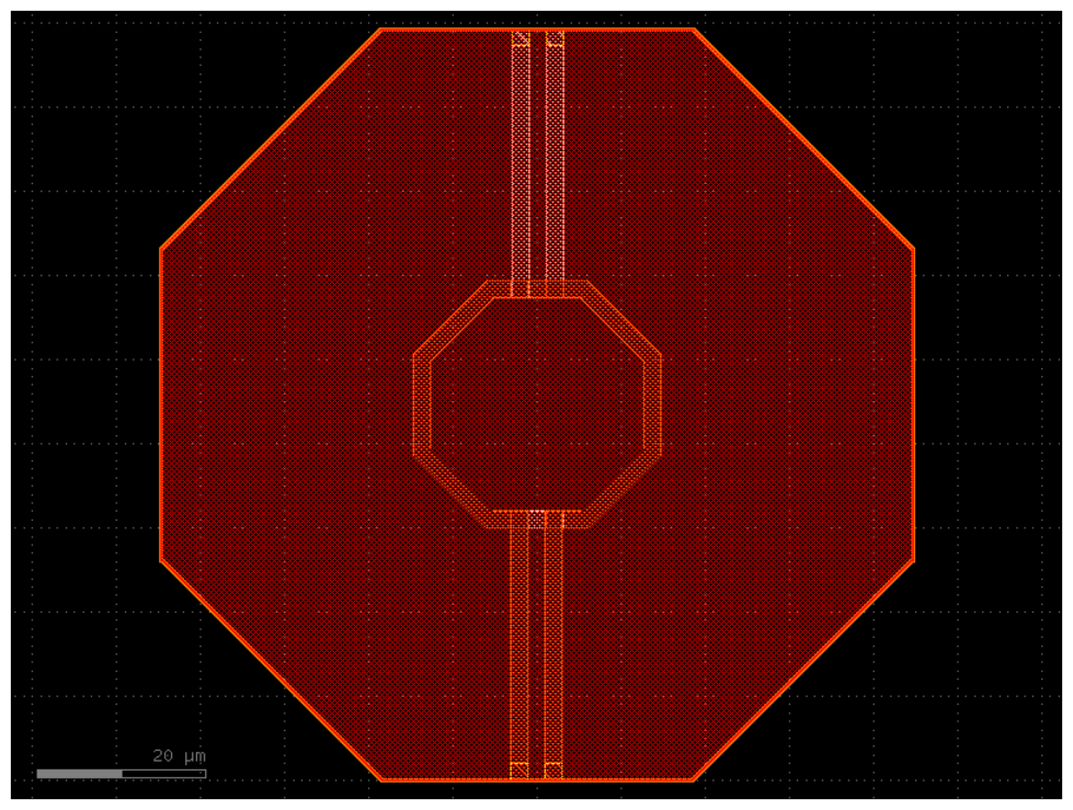
single-turn coils of the IHP SG13G2 PDK (inductor2):
- a coupled pair, one coil on TopMetal2 over a copy on TopMetal1, which shows the workflow;
- a side-by-side pair on TopMetal2, whose mutual inductance is checked against an analytic reference;
- two concentric rings, checked against closed-form inductances.
Requirements:
- ihp-gdsfactory==2.0.1
- A Palace backend: a GDSFactory+ account for cloud simulation (sim.run()), or a local
palace executable (sim.run_local()).
Model and material overrides
The IHP material values are unchanged; the model makes these choices:
- Conductors are perfect conductors. Palace's magnetostatic solver carries current only on perfect-conductor surfaces, so the metal conductivities are not used. The result is the external inductance, the high-frequency limit: the current flows on the metal surfaces, with no internal inductance and no resistance.
- No magnetic materials. The IHP material cards carry no permeability, so μr = 1 everywhere.
- No substrate.
set_stack()leaves it out by default. Doped silicon is not magnetic, and a static solve has no eddy currents, so it would only add mesh. - No guard ring, shield or fill. A closed metal loop that carries no source screens the field.
inductor2draws none; its marker layers (INDdrawing, the nofill layers) are not meshed.
The cell's c.info["inductance"] (33.3 pH) is a value passed through to the schematic, not a model of the
geometry, so it is not a reference here.
import gdsfactory as gf
import numpy as np
from ihp import PDK, cells

from gsim.palace import MagnetostaticSim

PDK.activate()


@gf.cell
def inductor2_pair(pitch: float = 39.35, stacked: bool = False) -> gf.Component:
    """Two single-turn inductor2 coils, ports A_P1/A_P2 and B_P1/B_P2.

    Coil A is on TopMetal2. With stacked=True, coil B is a TopMetal1 copy rotated
    180 degrees about the octagon centre, coaxial with A; otherwise it is a
    TopMetal2 copy `pitch` um to the right.
    """
    c = gf.Component()
    a = c << cells.inductor2()
    if stacked:
        b = c << cells.inductor2(
            layer_metal_2="TopMetal1drawing", layer_metal_2_pin="TopMetal1pin"
        )
        b.rotate(180, center=(0, 44.675))
    else:
        b = c << cells.inductor2()
        b.movex(pitch)
    c.add_ports(a.ports, prefix="A_")
    c.add_ports(b.ports, prefix="B_")
    return c
Coupled coils
Coil B sits 5.3 µm below coil A and is rotated by 180°, so its leads run clear of A's. Each coil gets one current
source between its two leads: a unit current enters at P1, runs round the coil and leaves at P2. gsim closes the
loop with a sheet across the 2.1 µm gap between the lead tips.
sim = MagnetostaticSim()
sim.set_output_dir("./palace-sim-magnetostatic")
sim.set_geometry(coupled)
sim.set_stack()
# Keep the outer wall far from the coils: it biases the inductance.
sim.set_airbox(margin_x=100, margin_y=100, z_above=150, z_below=150)
sim.add_current_source("A", plus_port="A_P1", minus_port="A_P2")
sim.add_current_source("B", plus_port="B_P1", minus_port="B_P2")

for source in sim.resolve_current_sources():
    print(source.name, source.layer, source.center, source.direction)
print(sim.validate_config())
A topmetal2 (0.0, 0.0) -X
B topmetal1 (0.0, 89.35000000000001) +X
Validation: PASSED
The mesh is graded from 1 µm at the metal (half the 2 µm trace width) to 30 µm in the air. fmax has no effect on a
static solve.
Mesh Summary
========================================
Dimensions: 229.4 x 289.4 x 317.9 µm
Nodes:      9,335
Elements:   68,566
Tetrahedra: 52,069
Edge length: 0.43 - 63.70 µm
Quality:    0.654 (min: 0.021)
SICN:       0.702 (all valid)
Worst element distortion, κ: 102.003 (tet centers; 1 is ideal)
Estimated Field DOFs: 333,806 (order 2; before Palace preprocessing)
Mesh hash:  sha256:44d0e5faa9d6b73e  (gmsh 4.15.2, gsim 0.10.0)
Mesher:     2D algorithm 5, 3D algorithm 1, threads 1 (1D/2D/3D limits 1/1/1)
----------------------------------------
Volumes (3):
  - sio2 [1]
  - sin [2]
  - air [3]
Surfaces (10):
  - topmetal1_xy [4]
  - topmetal1_z [5]
  - topmetal2_xy [6]
  - topmetal2_z [7]
  - P1 [8]
  - P2 [9]
  - air__sio2 [10]
  - sin__sio2 [11]
  - air__sin [12]
  - air__None [13]
----------------------------------------
Mesh:   palace-sim-magnetostatic/palace.msh
Run and read the matrix
check_cache=True reuses a finished cloud job with the same inputs. load_inductance labels the matrix with the
source names, and reads Palace's log to refuse a solve that did not converge, since such a solve still writes a
matrix that can look plausible. problems() lists what is physically inconsistent (reciprocity, energy, |k| ≤ 1); it
is empty here.
results = sim.run(check_cache=True)
inductance = sim.load_inductance(results)

print("Inductance matrix (pH):")
print((inductance.inductance_frame() * 1e12).round(3))
print("\nCoupling coefficients:")
print(inductance.coupling_frame().round(4))
print("\nConsistency checks:", inductance.problems() or "ok")
  palace-e400a769  [####################]  Job completed  elapsed 0m 00s


Extracting results.tar.gz...
Downloaded 13 files to sim-data-palace-e400a769
Inductance matrix (pH):
        A       B
A  50.104  19.227
B  19.227  55.307

Coupling coefficients:
        A       B
A  1.0000  0.3652
B  0.3652  1.0000

Consistency checks: ok
pairs = inductance.pairs()
pairs["inductance_pH"] = pairs["inductance_H"] * 1e12
pairs[["first", "second", "inductance_pH", "coupling"]].round(4)
| first | second | inductance_pH | coupling | |
|---|---|---|---|---|
| 0 | A | A | 50.1039 | 1.0000 |
| 1 | B | B | 55.3068 | 1.0000 |
| 2 | A | B | 19.2267 | 0.3652 |
For scale, the Neumann formula for the two centrelines gives M ≈ 19.3 pH. The mutual is positive: the coils are wound
the same way, so their fluxes add. Swapping plus_port and minus_port of one source flips the sign of its row and
column and leaves the self inductances unchanged.
Validation: two coils side by side
Two TopMetal2 coils at a 39.35 µm pitch (a 10 µm gap) have a small negative mutual inductance: the return flux of one coil threads the other backwards. Its references:
- Centreline filaments. The Neumann formula over the two coil centrelines gives −1.086 pH. Moving both filaments to the inner or the outer edges of the 2 µm traces gives −0.705 and −1.606 pH: the result depends strongly on where the current flows across the trace.
- PEC bundle. A perfect conductor carries its current on the trace surface, crowded towards the inside of the
loop and towards the other lead. Each coil then encloses about 6 % less area, which lowers |M| by about 11 %.
Modelling each trace as filaments on its surface, with the current split that a perfect conductor takes (the one
of least magnetic energy), gives −0.9606 pH in open space and L = 52.48 pH. These values are quoted here;
scripts/magnetostatic_pec_bundle.pyin the repository computes them in a few minutes. - Outer wall. The outer wall of the domain acts as an image of each coil behind each of its six faces, a series that converges slowly. As for the rings below, the pair is run with a PEC and with a PMC wall: their images have opposite signs, so the mean of the two runs cancels the first-order wall error. Second-order images, reflected in two walls, have the same sign for both walls and stay in the mean.
The check passes when the PEC/PMC mean is within 3 % of the PEC-bundle reference on both M and L. The mesh is finer here (0.5 µm at the metal) and the solve uses the default Order 2.
@gf.cell
def side_by_side() -> gf.Component:
    """Two TopMetal2 coils at a 39.35 um pitch."""
    return inductor2_pair(pitch=39.35)


def pair_sim(metallic_boundaries: bool, output_dir: str) -> MagnetostaticSim:
    """The side-by-side coils, one source each, in a box 100 um clear of them."""
    sim = MagnetostaticSim(metallic_boundaries=metallic_boundaries)
    sim.set_output_dir(output_dir)
    sim.set_geometry(side_by_side())
    sim.set_stack()
    sim.set_airbox(margin_x=100, margin_y=100, z_above=150, z_below=150)
    sim.add_current_source("A", plus_port="A_P1", minus_port="A_P2")
    sim.add_current_source("B", plus_port="B_P1", minus_port="B_P2")
    sim.mesh(refined_mesh_size=0.5, max_mesh_size=30.0)
    return sim


pair_pec = pair_sim(True, "./palace-sim-magnetostatic-pair-pec")
pair_pmc = pair_sim(False, "./palace-sim-magnetostatic-pair-pmc")
pair_runs = [
    sim.load_inductance(sim.run(check_cache=True)) for sim in (pair_pec, pair_pmc)
]
pair_matrix = (pair_runs[0].matrix + pair_runs[1].matrix) / 2
print(
    "PEC and PMC problems:",
    pair_runs[0].problems() or "ok",
    pair_runs[1].problems() or "ok",
)
for label, run in zip(("PEC", "PMC"), pair_runs, strict=True):
    print(f"{label} wall (pH):")
    print((run.inductance_frame() * 1e12).round(4))
  palace-218b5cd7  [####################]  Job completed  elapsed 0m 00s


Extracting results.tar.gz...
Downloaded 13 files to sim-data-palace-218b5cd7
PEC and PMC problems: ok ok
PEC wall (pH):
         A        B
A  51.2301  -0.9964
B  -0.9964  51.2321
PMC wall (pH):
         A        B
A  51.2674  -0.9615
B  -0.9615  51.2694
The filament reference: the Neumann double integral of dl·dl′/r over two closed paths, with Gauss-Legendre points on
pieces of at most 1 µm. offset shifts a path towards the loop interior (the inner trace edge is 1 µm in).
CENTRE_Y, APOTHEM, LEAD_X, Z_MID = 44.675, 13.675, 2.05, 12.53  # um, TopMetal2


def offset(path, u):
    """Shift an open, clockwise polyline by u um towards the loop interior."""
    t = np.diff(path, axis=0)
    t /= np.linalg.norm(t, axis=1)[:, None]
    n = np.c_[t[:, 1], -t[:, 0]]
    out = path.copy()
    out[0] += u * n[0]
    out[-1] += u * n[-1]
    for k in range(1, len(path) - 1):
        out[k] += u * (n[k - 1] + n[k]) / (1 + n[k - 1] @ n[k])
    return out


def coil(x0=0.0, u=0.0):
    """Closed current path of one coil, P1 -> octagon -> P2 -> P1, as 3D points (um)."""
    r = APOTHEM / np.cos(np.pi / 8)
    angles = np.deg2rad(22.5 + 45 * np.array([5, 4, 3, 2, 1, 0, 7, 6]))
    octagon = np.c_[r * np.cos(angles), CENTRE_Y + r * np.sin(angles)]
    y0 = CENTRE_Y - APOTHEM
    leads = np.array([(-LEAD_X, 0), (-LEAD_X, y0), *octagon, (LEAD_X, y0), (LEAD_X, 0)])
    path = offset(leads, u)
    path = np.c_[path[:, 0] + x0, path[:, 1], np.full(len(path), Z_MID)]
    return np.vstack([path, path[:1]])


def quadrature(path, h=1.0):
    """Gauss-Legendre points and weighted tangents, 4 per piece of at most h um."""
    x, w = np.polynomial.legendre.leggauss(4)
    points, tangents = [], []
    for a, b in zip(path[:-1], path[1:], strict=True):
        k = int(np.ceil(np.linalg.norm(b - a) / h))
        t = ((np.arange(k)[:, None] + (x + 1) / 2) / k).ravel()
        points.append(a + t[:, None] * (b - a))
        tangents.append(np.tile(w / (2 * k), k)[:, None] * (b - a))
    return np.vstack(points), np.vstack(tangents)


def neumann(a, b):
    """Mutual inductance of two closed filaments in um, in H."""
    (pa, da), (pb, db) = quadrature(a), quadrature(b)
    r = np.linalg.norm(pa[:, None] - pb[None], axis=-1)
    return 1e-7 * 1e-6 * np.sum((da @ db.T) / r)  # mu0/4pi, um -> m
PITCH = 39.35
M_BUNDLE = -0.9606e-12  # H, PEC bundle, open space
L_BUNDLE = 52.48e-12  # H, PEC bundle, open space

a, b = coil(), coil(PITCH)
m_centreline = neumann(a, b)
m_inner = neumann(coil(u=1.0), coil(PITCH, u=1.0))
m_outer = neumann(coil(u=-1.0), coil(PITCH, u=-1.0))

m_pec, m_pmc = (run.mutual_inductance("A", "B") for run in pair_runs)
m_palace = pair_matrix[0, 1]
wall = (m_pec - m_pmc) / 2 / m_palace
error_m = m_palace / M_BUNDLE - 1
in_bracket = min(m_inner, m_outer) < m_palace < max(m_inner, m_outer)
errors_l = [pair_matrix[k, k] / L_BUNDLE - 1 for k in range(2)]
coupling = m_palace / np.sqrt(pair_matrix[0, 0] * pair_matrix[1, 1])

pH = 1e12
print(f"Centreline Neumann:         {m_centreline * pH:.4f} pH")
print(f"Edge bracket (inner/outer): {m_inner * pH:.4f} / {m_outer * pH:.4f} pH")
print(f"PEC bundle reference:       {M_BUNDLE * pH:.4f} pH")
print(f"Palace M_AB, PEC / PMC:     {m_pec * pH:.4f} / {m_pmc * pH:.4f} pH")
print(f"  wall effect:              {wall:+.2%} (PEC), {-wall:+.2%} (PMC)")
print(f"Palace M_AB, mean:          {m_palace * pH:.4f} pH")
print(f"  vs PEC bundle:            {error_m:+.2%}")
print(f"  inside the edge bracket:  {in_bracket}")
print(f"  vs centreline:            {m_palace / m_centreline - 1:+.2%}")
print(f"Palace L_A, L_B vs bundle:  {errors_l[0]:+.2%}, {errors_l[1]:+.2%}")
print(f"Coupling k_AB:              {coupling:.4f}")

assert abs(error_m) <= 0.03
assert all(abs(error) <= 0.03 for error in errors_l)
Centreline Neumann:         -1.0857 pH
Edge bracket (inner/outer): -0.7050 / -1.6059 pH
PEC bundle reference:       -0.9606 pH
Palace M_AB, PEC / PMC:     -0.9964 / -0.9615 pH
  wall effect:              +1.78% (PEC), -1.78% (PMC)
Palace M_AB, mean:          -0.9789 pH
  vs PEC bundle:            +1.91%
  inside the edge bracket:  True
  vs centreline:            -9.84%
Palace L_A, L_B vs bundle:  -2.35%, -2.34%
Coupling k_AB:              -0.0191
The two walls move M_AB by about ±1.8 %, close to what the first-order images predict, and their mean removes that term. What remains is the comparison with the bundle.
Palace's self inductances lie about 2.3 % below the bundle. A conforming finite-element solution underestimates the stored energy, so the mesh error comes from below; the bundle is itself approximate (a ribbon model extrapolated to zero ribbon width), so part of the gap may be its own. The centreline formula overestimates |M| by about 10 %: it puts the current on the trace centre rather than on the crowded surface.
This M_AB is a small difference of large fluxes (k ≈ 0.02). Its |M| stays about 2 % above the open-space bundle and does not approach it as the mesh refines. The mean cancels only the first-order wall term, so part of this residual may be the second-order images; the rest is not yet explained. The check shows the right size and sign but not convergence. The next check does, on a pair whose answer has a closed form.
Validation: two concentric rings
Two coplanar rings of the same 2 × 3 µm section, with radii of 25 and 50 µm, have closed-form inductances:
- Self inductance. A slender perfect-conductor ring has L = μ₀R (ln(8R/a) − 2), where a is the radius of the round wire with the same external field. For a rectangle, a is its logarithmic capacity, from the Schwarz-Christoffel map of the section: 1.469 µm here.
- Mutual inductance. Maxwell's formula for two coaxial circles, with elliptic integrals of modulus k² = 4R₁R₂ / (R₁ + R₂)².
Both hold for thin rings. To quantify what thinness leaves out, the rings are also compared with a ribbon bundle on
the trace surface, as for the coils above, whose mutual inductances are all Maxwell's formula. It needs no finite
elements: scripts/magnetostatic_pec_bundle.py gives L = 91.25 and 226.08 pH and M = 27.106 pH. Its M lies 1.2 % below
the thin-ring formula, since a perfect conductor crowds the current on the faces of the trace.
A cut of 1 µm in each ring carries the current source. Each ring is a 96-sided polygon, which encloses 0.07 % less area than the circle. Rather than model the outer wall, the check runs it both ways and takes the mean of a PEC and a PMC wall, which cancels its first-order error.
from scipy.integrate import quad
from scipy.optimize import brentq
from scipy.special import ellipe, ellipk

R_A, R_B = 25.0, 50.0  # um
WIDTH, THICKNESS = 2.0, 3.0  # um, TopMetal2
MU0 = 4e-7 * np.pi  # H/m


@gf.cell
def split_ring(radius: float, gap: float = 1.0, sides: int = 96) -> gf.Component:
    """A ring cut by a gap on the +x axis, with its two ports facing across the gap."""

    def arc(r):
        start = np.arcsin(gap / 2 / r)
        angles = np.linspace(start, 2 * np.pi - start, sides + 1)
        return np.c_[r * np.cos(angles), r * np.sin(angles)]

    c = gf.Component()
    c.add_polygon(
        np.vstack([arc(radius + WIDTH / 2), arc(radius - WIDTH / 2)[::-1]]),
        layer="TopMetal2drawing",
    )
    for name, y, orientation in (("plus", -gap / 2, 90), ("minus", gap / 2, 270)):
        c.add_port(
            name,
            center=(radius, y),
            width=WIDTH,
            orientation=orientation,
            layer="TopMetal2drawing",
            port_type="electrical",
        )
    return c


@gf.cell
def concentric_rings() -> gf.Component:
    """Two concentric split rings, ports A_plus/A_minus and B_plus/B_minus."""
    c = gf.Component()
    c.add_ports((c << split_ring(R_A)).ports, prefix="A_")
    c.add_ports((c << split_ring(R_B)).ports, prefix="B_")
    return c


def rings_sim(metallic_boundaries: bool, output_dir: str) -> MagnetostaticSim:
    """The rings with one source each, in a box 150 um clear of them."""
    sim = MagnetostaticSim(metallic_boundaries=metallic_boundaries)
    sim.set_output_dir(output_dir)
    sim.set_geometry(concentric_rings())
    sim.set_stack()
    sim.set_airbox(margin_x=150, margin_y=150, z_above=150, z_below=150)
    sim.add_current_source("A", plus_port="A_plus", minus_port="A_minus")
    sim.add_current_source("B", plus_port="B_plus", minus_port="B_minus")
    sim.mesh(refined_mesh_size=0.5, max_mesh_size=30.0)
    return sim


rings_pec = rings_sim(True, "./palace-sim-magnetostatic-rings-pec")
rings_pmc = rings_sim(False, "./palace-sim-magnetostatic-rings-pmc")
ring_runs = [
    sim.load_inductance(sim.run(check_cache=True)) for sim in (rings_pec, rings_pmc)
]
rings_matrix = (ring_runs[0].matrix + ring_runs[1].matrix) / 2
print(
    "PEC and PMC problems:",
    ring_runs[0].problems() or "ok",
    ring_runs[1].problems() or "ok",
)
print("PEC/PMC mean (pH):")
print((rings_matrix * 1e12).round(3))
  palace-da9dc022  [####################]  Job completed  elapsed 0m 00s


Extracting results.tar.gz...
Downloaded 13 files to sim-data-palace-da9dc022
PEC and PMC problems: ok ok
PEC/PMC mean (pH):
[[ 90.859  27.06 ]
 [ 27.06  225.073]]
def equivalent_radius(width, thickness):
    """Logarithmic capacity of a rectangle, from its Schwarz-Christoffel map."""

    def sides(theta):
        cosine = np.cos(2 * theta)
        short = quad(lambda p: np.sqrt(2 * (np.cos(2 * p) - cosine)), -theta, theta)
        long = quad(
            lambda p: np.sqrt(2 * (cosine - np.cos(2 * p))), theta, np.pi - theta
        )
        return short[0], long[0]

    aspect = min(width, thickness) / max(width, thickness)
    theta = brentq(lambda t: sides(t)[0] / sides(t)[1] - aspect, 1e-6, np.pi / 2 - 1e-6)
    return max(width, thickness) / sides(theta)[1]


def ring_self(radius, a):
    """Self inductance of a slender perfect-conductor ring, radii in um, in H."""
    return MU0 * radius * 1e-6 * (np.log(8 * radius / a) - 2)


def maxwell(first, second):
    """Mutual inductance of two coplanar coaxial circles, radii in um, in H."""
    m = 4 * first * second / (first + second) ** 2
    k = np.sqrt(m)
    return (
        MU0
        * np.sqrt(first * second)
        * 1e-6
        * ((2 / k - k) * ellipk(m) - 2 / k * ellipe(m))
    )


a_eq = equivalent_radius(WIDTH, THICKNESS)
closed = np.array(
    [
        [ring_self(R_A, a_eq), maxwell(R_A, R_B)],
        [maxwell(R_A, R_B), ring_self(R_B, a_eq)],
    ]
)
RIBBONS = np.array([[91.25, 27.106], [27.106, 226.08]]) * 1e-12  # H, see above

print(f"Equivalent radius: {a_eq:.4f} um")
for label, row, column in (("L_A", 0, 0), ("L_B", 1, 1), ("M_AB", 0, 1)):
    palace = rings_matrix[row, column]
    print(
        f"{label:<5} Palace {palace * 1e12:8.3f} pH | "
        f"closed form {closed[row, column] * 1e12:8.3f} pH ({palace / closed[row, column] - 1:+.2%}) | "
        f"ribbons {RIBBONS[row, column] * 1e12:8.3f} pH ({palace / RIBBONS[row, column] - 1:+.2%})"
    )

assert np.all(np.abs(rings_matrix / closed - 1) <= 0.02)
assert np.all(np.abs(rings_matrix / RIBBONS - 1) <= 0.01)
Equivalent radius: 1.4692 um
L_A   Palace   90.859 pH | closed form   91.533 pH (-0.74%) | ribbons   91.250 pH (-0.43%)
L_B   Palace  225.073 pH | closed form  226.618 pH (-0.68%) | ribbons  226.080 pH (-0.45%)
M_AB  Palace   27.060 pH | closed form   27.431 pH (-1.35%) | ribbons   27.106 pH (-0.17%)
Palace agrees with the closed forms within 2 % and with the ribbon bundle within 1 %. The 1 % bound was set after these runs, so it serves as a regression gate rather than an independent tolerance. Refining the conductor mesh of the PEC run from 1 to 0.35 µm takes its self inductances from 1.0 % and 0.8 % below the reference to 0.3 %, and its mutual from 0.18 % to 0.13 % below, against the bundle with the wall effect from the PEC/PMC runs. Unlike the coils above, these errors shrink with the mesh and come from below, as a conforming solution should.
The cut is part of each loop: gsim replaces the metal across it by the source sheet, so its width changes the inductance. Keep the gap small against the loop.
Notes
- Outer wall bracket.
MagnetostaticSim(metallic_boundaries=False)makes the outer wall a perfect magnetic conductor. A PEC and a PMC run bracket the open-space value: an energy bound for the self inductances, a first-order bracket for the mutuals. Their mean cancels the first-order wall error; second-order images remain. - Mesh convergence. With Palace v0.18.1 at Order 2, refining the conductor mesh of the side-by-side pair from 0.7 to 0.5 µm changed M_AB by 0.18 % and the self inductances by 0.4 %.