FEM Dataset Lookup in SAX Models#

Required extras

This notebook needs the models extra:

uv add "qpdk[models]"
# or, from a checkout of this repository:
uv sync --extra models
# or with pip:
pip install "qpdk[models]"

See the extras reference for what each extra installs.

Circuit models of superconducting layouts need electrostatic quantities such as capacitance matrices, which for realistic geometries come from finite-element (FEM) solvers [Jin14]. One solve takes minutes to hours, far too slow to call inside a circuit simulation or an optimisation loop. So a sweep over the design parameters is solved once, stored as a dataset, and the circuit model interpolates between the stored points.

        flowchart TB
    A["FEM solve<br/>per geometry"] --> B["Sweep over<br/>parameter grid"]
    B --> C["Parquet parts or<br/>Delta table + metadata"]
    C --> D["Dataset.grid<br/>dense array"]
    D --> E["GridInterpolator<br/>jittable lookup"]
    E --> F["SAX model"]

qpdk.models.datasets stores the results as a long-format Polars table with one row per matrix entry. Each Parquet file (or the Delta table schema) also carries the dataset metadata: units, terminal and ground conventions, whether the data is synthetic, and free-form provenance such as the layer stack and solver. A file is therefore self-describing, and the parameter grid is read off the data rather than declared separately. Curated datasets ship in the package as Parquet parts in Git LFS; shared, growing datasets can live in a Delta Lake table on a cloud bucket.

This notebook follows generation, storage, lazy queries and JAX interpolation, then uses the capacitance lookup in a SAX model. Run uv run --script notebooks/src/fem_dataset_lookup.py with Git LFS installed to use the pinned QPDK revision and fetch its bundled results automatically.

The bundled data comes from Palace electrostatic solves of the actual QPDK metal polygons, including their short leads, as perfect conductor sheets on silicon. A separate coplanar ground frame surrounds the device. The geometry and mesh settings travel with the data. It covers lengths 40–120 µm, widths 5–20 µm and gaps 4–10 µm; these results apply to that geometry and stack.

Inspect the dataset#

The metadata is read from the files and validated when the dataset opens. The results table is a plain Polars frame with one row per matrix entry, so it can be filtered and aggregated without loading anything into JAX.

dataset = Dataset("plate_capacitor_palace")
metadata = dataset.metadata
logger.info(f"{dataset!r}: synthetic={metadata.synthetic}")
logger.info(f"solver: {metadata.provenance['solver']}")
logger.info(f"extraction settings: {metadata.provenance['settings']}")
logger.info(f"terminals {metadata.terminals} w.r.t. {metadata.reference_ground!r}")
for axis in metadata.axes:
    logger.info(
        f"{axis.name} [{axis.unit}]: validated domain {axis.validated or 'grid span'}"
    )

2026-10-22 13:29:39.435 | INFO     | __main__:<module>:3 - Dataset('plate_capacitor_palace', store=ParquetParts('/home/runner/work/quantum-rf-pdk/quantum-rf-pdk/qpdk/models/datasets/data/plate_capacitor_palace')): synthetic=False

2026-10-22 13:29:39.436 | INFO     | __main__:<module>:4 - solver: Palace

2026-10-22 13:29:39.437 | INFO     | __main__:<module>:5 - extraction settings: {'near_mesh': 0.55, 'far_mesh': 25.0, 'domain_pad': 100.0, 'ground_clearance': 10.0, 'ground_pad': 45.0, 'permittivity': 11.45, 'order': 2, 'tolerance': 1e-09, 'save_fields': False}

2026-10-22 13:29:39.437 | INFO     | __main__:<module>:6 - terminals ('o1', 'o2') w.r.t. 'coplanar_ground_frame'

2026-10-22 13:29:39.438 | INFO     | __main__:<module>:8 - length [um]: validated domain grid span

2026-10-22 13:29:39.438 | INFO     | __main__:<module>:8 - width [um]: validated domain grid span

2026-10-22 13:29:39.439 | INFO     | __main__:<module>:8 - gap [um]: validated domain grid span

dataset.table.head(8)

shape: (8, 12)

run_id	status	length	width	gap	cross_section	quantity	row	col	value	value_imag	unit
str	str	f64	f64	f64	str	str	str	str	f64	f64	str
"b42beed1e26f12ae"	"ok"	40.0	5.0	4.0	"cpw"	"fem_error_indicator_norm"	null	null	0.281896	null	"1"
"b42beed1e26f12ae"	"ok"	40.0	5.0	4.0	"cpw"	"maxwell_capacitance"	"o1"	"o1"	6.5721e-15	null	"F"
"b42beed1e26f12ae"	"ok"	40.0	5.0	4.0	"cpw"	"maxwell_capacitance"	"o1"	"o2"	-2.2157e-15	null	"F"
"b42beed1e26f12ae"	"ok"	40.0	5.0	4.0	"cpw"	"maxwell_capacitance"	"o2"	"o1"	-2.2157e-15	null	"F"
"b42beed1e26f12ae"	"ok"	40.0	5.0	4.0	"cpw"	"maxwell_capacitance"	"o2"	"o2"	6.5759e-15	null	"F"
"b42beed1e26f12ae"	"ok"	40.0	5.0	4.0	"cpw"	"solver_iterations"	null	null	12.0	null	"1"
"b42beed1e26f12ae"	"ok"	40.0	5.0	4.0	"cpw"	"solver_relative_residual"	null	null	3.2135e-10	null	"1"
"a2293eecb392f6e3"	"ok"	40.0	5.0	7.0	"cpw"	"fem_error_indicator_norm"	null	null	0.271239	null	"1"

(
    dataset
    .scan()
    .filter(pl.col("row") != pl.col("col"))
    .group_by("gap")
    .agg(c_mutual_fF=(-pl.col("value")).mean() * 1e15)
    .sort("gap")
    .collect()
)

shape: (3, 2)

gap	c_mutual_fF
f64	f64
4.0	5.735053
7.0	4.348927
10.0	3.538881

Define a generation script#

qpdk/models/datasets/data/plate_capacitor.py is a complete experiment: its GRID, SETTINGS, metadata and solve function describe what to extract. Its inline dependencies let uv run --script create the Python 3.12 environment required by gsim. Copy the script beside the original in qpdk/models/datasets/data/ and edit it for another dataset.

Meshing runs on the host, including when Palace uses --sif. Gmsh needs its native libraries there; on Linux this includes libGLU.so.1. The container needs a Palace binary with MPI support; select its executable with --container-binary.

Preview the full sweep or run it from a checkout:

uv run --script qpdk/models/datasets/data/plate_capacitor.py --dry-run
uv run --script qpdk/models/datasets/data/plate_capacitor.py --processes 4
# A local Palace container:
uv run --script qpdk/models/datasets/data/plate_capacitor.py --sif /path/to/palace.sif

--processes sets CPU threads for meshing and MPI ranks for Palace. The script builds a QPDK component. gsim meshes its electrodes with meshwell, writes the configuration and runs Palace. Results carry their metadata; lookup needs neither the generator nor the simulator. Generator scripts stay outside wheels.

small_grid = {"length": [40.0, 80.0], "width": [10.0], "gap": [4.0, 7.0, 10.0]}
output = Path("build/dataset-example/coarse")
generator_script = Path("qpdk/models/datasets/data/plate_capacitor.py")

Run a small sweep and inspect its output#

Copy the generator beside the original, replace GRID with small_grid, then run it with --output build/dataset-example/coarse. For example, its grid definition becomes:

GRID = {"length": [40.0, 80.0], "width": [10.0], "gap": [4.0, 7.0, 10.0]}

Set RUN_PALACE=True to execute the generator from a checkout. It runs the grid defined in generator_script; point this path to your edited copy. The default selects six existing Palace results and performs no new solves. Both paths produce a self-describing table with four matrix entries and scalar diagnostics per solve.

RUN_PALACE = False

if RUN_PALACE:
    subprocess.run(  # ruff: ignore[subprocess-without-shell-equals-true]
        [
            "uv",
            "run",
            "--script",
            str(generator_script),
            "--output",
            str(output),
        ],
        check=True,
    )
    generated = Dataset(output)
else:
    selection = (
        dataset
        .scan()
        .filter(*(pl.col(axis).is_in(values) for axis, values in small_grid.items()))
        .collect()
    )
    generated = write(output, dataset.metadata, selection)
    logger.info("Selected six existing Palace solves; no simulator was run")
coarse = generated.grid("maxwell_capacitance", cross_section="cpw")
logger.info(f"Output: {generated.scan().select(pl.len()).collect().item()} rows")
logger.info(
    f"Dense grid: {coarse.values.shape}, terminals={generated.metadata.terminals}"
)
coarse_lookup = GridInterpolator(coarse)
logger.info(
    f"Small-sweep lookup at 60/10/7 µm [fF]:\n"
    f"{coarse_lookup(length=60.0, width=10.0, gap=7.0) * 1e15}"
)

2026-10-22 13:29:39.504 | INFO     | __main__:<module>:24 - Selected six existing Palace solves; no simulator was run

2026-10-22 13:29:39.517 | INFO     | __main__:<module>:26 - Output: 42 rows

2026-10-22 13:29:39.517 | INFO     | __main__:<module>:27 - Dense grid: (2, 1, 3, 2, 2), terminals=('o1', 'o2')

2026-10-22 13:29:40.576 | INFO     | __main__:<module>:31 - Small-sweep lookup at 60/10/7 µm [fF]:
[[10.89142216 -3.13709128]
 [-3.13709128 10.90180517]]

(
    generated
    .scan()
    .filter(pl.col("quantity") == "maxwell_capacitance")
    .group_by("length", "width", "gap", "status")
    .len(name="matrix_entries")
    .sort("length", "gap")
    .collect()
)

shape: (6, 5)

length	width	gap	status	matrix_entries
f64	f64	f64	str	u32
40.0	10.0	4.0	"ok"	4
40.0	10.0	7.0	"ok"	4
40.0	10.0	10.0	"ok"	4
80.0	10.0	4.0	"ok"	4
80.0	10.0	7.0	"ok"	4
80.0	10.0	10.0	"ok"	4

Resume and extend a sweep#

Rerun the generator after an interruption. Each geometry retains its inputs, mesh, config, solver log and output. Completed matching runs are reused; failed ones retry. Geometry, mesh, generator or runtime changes get a new run directory. The published dataset is replaced only after the sweep succeeds.

Add 120.0 to the small script’s length grid and rerun with the same --workdir: six geometries are reused and three are added. Use --output and --workdir to select locations; paths are relative to your current directory.

Parallel sweeps#

Both experiments accept --shard INDEX --shards COUNT. The longest axis is split into disjoint rectangular grids, with unchanged solver inputs and run identities. Workers write separate outputs and run directories; merging checks provenance, coverage and successful results before publication. Use a small array of longer shards, with no more tasks than points on the longest axis. For the CPW grid:

generator=qpdk/models/datasets/data/cpw_coupling.py
sbatch --array=0-1 --cpus-per-task=4 qpdk/models/datasets/data/slurm_array.sh "$generator" \
  build/cpw-shards build/cpw-runs --sif /path/to/palace.sif
# After every task succeeds, pass each shard as a repeated option:
shards=()
for i in {0..1}; do shards+=(--merge-shards "build/cpw-shards/shard-$i"); done
uv run --script "$generator" "${shards[@]}" --output build/datasets/cpw_coupling_palace

Each task runs one solve at a time with four MPI ranks, one thread per rank. Specify the array size with --array; --cpus-per-task sets MPI ranks per solve.

Without Slurm, run the entire script directly or use a local loop. This sequential loop needs four cores; independent shard commands can also run concurrently if each has its own four-core allocation:

generator=qpdk/models/datasets/data/cpw_coupling.py
export OMP_NUM_THREADS=1 OPENBLAS_NUM_THREADS=1 MKL_NUM_THREADS=1
shards=()
for i in {0..1}; do
  uv run --script "$generator" --shard "$i" --shards 2 --processes 4 \
    --output "build/cpw-shards/shard-$i" --workdir "build/cpw-runs/shard-$i"
  shards+=(--merge-shards "build/cpw-shards/shard-$i")
done
uv run --script "$generator" "${shards[@]}" --output build/datasets/cpw_coupling_palace

Keep the script, settings, runtime and array size fixed while resuming. The reusable partition_grid and merge functions also work with other experiment scripts and schedulers.

Check mesh and domain sensitivity#

Each result stores the worst terminal’s linear-solver residual and iteration count, plus Palace’s energy-normalized recovered-flux FEM error indicator. The generator rejects missing diagnostics or a linear solve that exceeds SETTINGS.tolerance. Linear convergence alone does not establish mesh accuracy. The FEM indicator ranks candidates for refinement; it is not a percentage error in capacitance.

A denser parameter grid cannot repair a coarse FEM mesh. In a copy of the generator, select one geometry and vary the settings:

from dataclasses import replace

GRID = {"length": [80.0], "width": [10.0], "gap": [7.0]}
SETTINGS = replace(SETTINGS, near_mesh=0.38, far_mesh=17.0, save_fields=True)

Reduce both near and far mesh sizes with separate output directories, then increase domain_pad to 150 µm. Compare the Maxwell matrices and inspect the saved fields in ParaView, especially near metal edges and gaps. Repeat representative checks near the ends of any expanded geometry range. For each quantity of interest, compare successive solves using \(|C_{\text{fine}}-C_{\text{coarse}}|/|C_{\text{fine}}|\), checking mesh and domain changes separately.

The bundled plate dataset records representative finer-mesh and larger-domain comparisons, a native-runtime cross-check and fresh off-grid references in its provenance. These finite checks do not establish a uniform accuracy bound.

plate_checks = metadata.provenance["validation"]
logger.info(
    f"Native runtime grid comparison: {plate_checks['native_grid_max_relative']:.3%}; "
    f"{plate_checks['held_out_points']} off-grid references: "
    f"maximum lookup difference {plate_checks['held_out_max_relative']:.2%}"
)
(
    pl
    .DataFrame(plate_checks["mesh_domain"])
    .unnest("point")
    .select(
        "length",
        "width",
        "gap",
        (100 * pl.col("refined_relative")).alias("Finer mesh (%)"),
        (100 * pl.col("domain_relative")).alias("Larger domain (%)"),
    )
)

2026-10-22 13:29:40.592 | INFO     | __main__:<module>:2 - Native runtime grid comparison: 0.000%; 4 off-grid references: maximum lookup difference 2.79%

shape: (3, 5)

length	width	gap	Finer mesh (%)	Larger domain (%)
f64	f64	f64	f64	f64
40.0	5.0	4.0	0.73666	0.1187
80.0	10.0	7.0	0.782793	0.168654
120.0	20.0	10.0	0.776481	0.282732

Query a shared Delta table#

Cloud datasets use the same interface. Select the quantity and variant before collecting; grid() does this internally. Pin a version for reproducible models:

shared = Dataset("gs://my-bucket/capacitors", delta=True, version=3)
rows = shared.scan().filter(
    pl.col("quantity") == "maxwell_capacitance",
    pl.col("cross_section") == "cpw",
).select("length", "gap", "value").collect()
lookup = GridInterpolator(shared.grid("maxwell_capacitance", cross_section="cpw"))

Scans stay lazy until collect(), allowing Polars to push filters and column selection into storage. Only the selected interpolation grid becomes a dense in-memory array. dataset.table explicitly loads and validates all rows.

Look up a Maxwell capacitance matrix#

For conductors \(1, \dots, n\) at potentials \(V_j\) above a reference ground, the charges are linear in the potentials, \(Q_i = \sum_j C_{ij} V_j\). The Maxwell capacitance matrix \(C\) is what an electrostatic FEM solver returns: it is symmetric, its diagonal is positive, and its off-diagonal entries are non-positive. The mutual capacitance between conductors \(i \neq j\) is \(C^{\text{m}}_{ij} = -C_{ij}\), and the capacitance of conductor \(i\) to ground is the row sum \(C^{\text{m}}_{ii} = \sum_j C_{ij}\). The mutual form is what appears as branch capacitances in a lumped circuit, and the Maxwell form is the capacitance matrix of circuit quantization [VD17]. maxwell_to_mutual() converts between them, and check_maxwell() raises if any property above is violated.

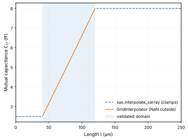
Between the solved points the lookup is multilinear: inside the grid cell containing a query, the result is a weighted mean of the \(2^n\) cell corners, with weights that are products of the 1D linear weights along each axis [WZ88]. It reproduces the data exactly at grid points, is continuous everywhere, and needs no tuning. Outside the validated domain there is no data to weigh, so the result is NaN.

grid() arranges the table into a dense (length, width, gap, 2, 2) array and raises if a grid point is missing or failed. Discrete variants such as the cross-section are chosen explicitly here and never interpolated. GridInterpolator wraps jax.scipy.interpolate.RegularGridInterpolator and holds plain JAX arrays, so it works inside jax.jit(), jax.vmap(), and jax.grad().

grid = dataset.grid("maxwell_capacitance", cross_section="cpw")
c_maxwell = GridInterpolator(grid)
logger.info(repr(c_maxwell))

C = c_maxwell(length=100.0, width=10.0, gap=5.0)
logger.info(f"Maxwell matrix [fF]:\n{C * 1e15}")
logger.info(f"Mutual matrix [fF]:\n{maxwell_to_mutual(C) * 1e15}")
check_maxwell(C)  # raises NonPhysicalMatrixError if C is not physical

2026-10-22 13:29:40.623 | INFO     | __main__:<module>:3 - GridInterpolator('plate_capacitor_palace', 'maxwell_capacitance', domain={'length': (40.0, 120.0), 'width': (5.0, 20.0), 'gap': (4.0, 10.0)}, out_of_range='nan')

2026-10-22 13:29:40.751 | INFO     | __main__:<module>:6 - Maxwell matrix [fF]:
[[17.73218645 -6.60501633]
 [-6.60501633 17.71842436]]

2026-10-22 13:29:40.990 | INFO     | __main__:<module>:7 - Mutual matrix [fF]:
[[11.12717012  6.60501633]
 [ 6.60501633 11.11340803]]

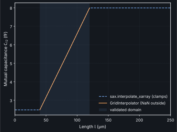
Outside the validated domain the lookup returns NaN. sax.interpolate_xarray() clamps to the nearest edge instead, which hides an out-of-range design.

lengths = jnp.linspace(0.0, 250.0, 251)
ours = -c_maxwell(length=lengths, width=10.0, gap=5.0)[:, 0, 1]

xarr = xr.DataArray(
    grid.values.reshape(*grid.values.shape[:3], 4),
    coords={
        **dict(zip(grid.axis_names, grid.coords, strict=True)),
        "targets": np.array(["c11", "c12", "c21", "c22"], dtype=object),
    },
)
theirs = -jax.vmap(
    lambda length: sax.interpolate_xarray(
        xarr, length=length, width=jnp.asarray(10.0), gap=jnp.asarray(5.0)
    )["c12"]
)(lengths)

fig, ax = plt.subplots()
ax.plot(lengths, theirs * 1e15, "--", label="sax.interpolate_xarray (clamps)")
ax.plot(lengths, ours * 1e15, label="GridInterpolator (NaN outside)")
ax.axvspan(*c_maxwell.domain["length"], alpha=0.1, label="validated domain")
ax.set_xlabel(r"Length $l$ ($\text{µm}$)")
ax.set_ylabel(r"Mutual capacitance $C_{12}$ ($\text{fF}$)")
ax.legend()
plt.show()

../_images/2530ce94c00c452a5619df9910eb2f0812c4e73db4f03f81b467cd392334ecb9.svg

../_images/2530ce94c00c452a5619df9910eb2f0812c4e73db4f03f81b467cd392334ecb9_dark.svg

Replace an explicit capacitance in a SAX model#

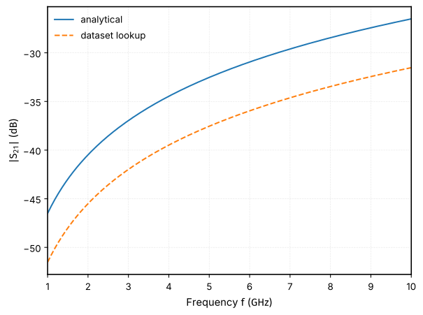
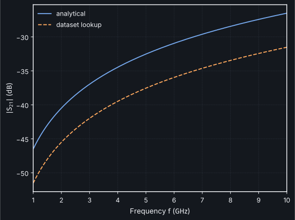
plate_capacitor() computes its capacitance from a closed-form expression. The same circuit can take the mutual capacitance from the dataset instead. The analytical formula and FEM model include different geometry and ground assumptions, so their disagreement is visible here. The lookup uses only the mutual branch; a complete circuit can also include the extracted pad-to-ground capacitances. capacitance_model supplies that complete lumped N-port network for any number of terminals; s_parameters_model directly interpolates stored N-port scattering data.

def plate_capacitor_lookup(
    *,
    f=DEFAULT_FREQUENCY,
    length: float = 80.0,
    width: float = 5.0,
    gap: float = 7.0,
    cross_section="cpw",
) -> sax.SDict:
    """Plate capacitor with the mutual capacitance looked up from the dataset."""
    f = jnp.asarray(f)
    c_mutual = maxwell_to_mutual(c_maxwell(length=length, width=width, gap=gap))[0, 1]
    return capacitor(
        f=f, capacitance=c_mutual, z0=cpw_z0_from_cross_section(cross_section, f)
    )


complete_plate = capacitance_model(dataset, cross_section="cpw")
logger.info(
    f"Complete two-terminal network at 5 GHz: "
    f"{complete_plate(f=5e9, length=80.0, width=10.0, gap=7.0)}"
)

f = jnp.linspace(1e9, 10e9, 201)
s_lookup = jax.jit(
    lambda gap: plate_capacitor_lookup(f=f, length=80.0, width=10.0, gap=gap)
)(7.0)
s_analytical = plate_capacitor(f=f, length=80.0, width=10.0, gap=7.0)

fig, ax = plt.subplots()
ax.plot(f / 1e9, 20 * jnp.log10(jnp.abs(s_analytical["o1", "o2"])), label="analytical")
ax.plot(
    f / 1e9, 20 * jnp.log10(jnp.abs(s_lookup["o1", "o2"])), "--", label="dataset lookup"
)
ax.set_xlabel(r"Frequency $f$ ($\text{GHz}$)")
ax.set_ylabel(r"$|S_{21}|$ ($\text{dB}$)")
ax.legend()
plt.show()

2026-10-22 13:29:46.130 | INFO     | __main__:<module>:18 - Complete two-terminal network at 5 GHz: {('o1', 'o1'): Array(0.9989619-0.04352421j, dtype=complex128), ('o1', 'o2'): Array(0.00058555+0.01343248j, dtype=complex128), ('o2', 'o1'): Array(0.00058555+0.01343248j, dtype=complex128), ('o2', 'o2'): Array(0.99895995-0.04356874j, dtype=complex128)}

../_images/97113106be373eb1e63603dc20c432da4d30ae40fc7de6f3cd9450e346334d5d.svg

../_images/97113106be373eb1e63603dc20c432da4d30ae40fc7de6f3cd9450e346334d5d_dark.svg

The lookup is differentiable, so the gap can be tuned by gradient descent towards a target transmission.

d_s21_d_gap = jax.jit(
    jax.grad(
        lambda gap: jnp.abs(
            plate_capacitor_lookup(f=5e9, length=80.0, width=10.0, gap=gap)["o1", "o2"]
        )
    )
)
logger.info(f"d|S21|/d gap at 5 GHz, gap = 7 µm: {float(d_s21_d_gap(7.0)):.3e} 1/µm")

2026-10-22 13:29:48.445 | INFO     | __main__:<module>:8 - d|S21|/d gap at 5 GHz, gap = 7 µm: -1.448e-03 1/µm

Compile and query time#

Compile time and steady-state query time are measured separately, for a single point and for a batch of 10 000 points.

def benchmark(fn, *args, repeats: int = 50) -> tuple[float, float]:
    """Return (compile time, steady-state time per call) in ms."""
    jitted = jax.jit(fn)
    t0 = time.perf_counter()
    jax.block_until_ready(jitted(*args))
    compile_ms = (time.perf_counter() - t0) * 1e3
    t0 = time.perf_counter()
    for _ in range(repeats):
        jax.block_until_ready(jitted(*args))
    return compile_ms, (time.perf_counter() - t0) / repeats * 1e3


rng = np.random.default_rng(0)
batch = {
    name: jnp.asarray(rng.uniform(lo, hi, 10_000))
    for name, (lo, hi) in c_maxwell.domain.items()
}
single = {name: x[0] for name, x in batch.items()}

rows = []
for label, point in [("1 point", single), ("10 000 points", batch)]:
    for method, fn in [
        ("GridInterpolator", lambda p: c_maxwell(**p)[..., 0, 1]),
        ("sax.interpolate_xarray", lambda p: sax.interpolate_xarray(xarr, **p)["c12"]),
    ]:
        compile_ms, query_ms = benchmark(fn, point)
        rows.append({
            "method": method,
            "query": label,
            "compile_ms": compile_ms,
            "query_ms": query_ms,
        })
pl.DataFrame(rows)

shape: (4, 4)

method	query	compile_ms	query_ms
str	str	f64	f64
"GridInterpolator"	"1 point"	255.055643	0.072672
"sax.interpolate_xarray"	"1 point"	182.441207	0.028726
"GridInterpolator"	"10 000 points"	289.342737	0.336759
"sax.interpolate_xarray"	"10 000 points"	312.985474	0.413262

Symmetric CPW coupling: a three-dimensional dataset#

qpdk/models/datasets/data/cpw_coupling.py follows the same workflow, sweeping trace width, outer CPW slot width and the gap between two identical traces. The inner gap is fully etched; there is no ground strip between the traces. Both conductors and the outer ground rails define a two-dimensional transverse Palace mesh, eliminating end fringing. Model.Lc sets the implicit slice depth; stored capacitances are in F for that depth. The lookup has three geometry axes.

uv run --script qpdk/models/datasets/data/cpw_coupling.py --dry-run
uv run --script qpdk/models/datasets/data/cpw_coupling.py --sif /path/to/palace.sif
uv run --script qpdk/models/datasets/data/cpw_coupling.py --topology as-drawn --sif /path/to/palace.sif

The generator refines every geometry until each raw Maxwell entry changes by at most 1% between successive meshes and identical traces agree within 1%. It stores the accepted finer matrix, mesh sizes, refinement level and measured change. This measures mesh sensitivity; it does not bound domain truncation or interpolation error. Separate domain, vacuum and held-out checks travel in the bundled dataset’s provenance. Solver matrices remain raw. The smaller development grid trades lookup resolution for faster regeneration; check its measured interpolation error before extending a design sweep.

The following cells read the bundled Palace results and run no simulator. The same interpolator handles all three axes; fixing an axis only chooses a view of that three-dimensional lookup.

cpw_dataset = Dataset("cpw_coupling_palace")
cpw_grid = cpw_dataset.grid("maxwell_capacitance")
cpw_lookup = GridInterpolator(cpw_grid)
slice_length = cpw_dataset.metadata.provenance["settings"]["slice_length_um"] * 1e-6
logger.info(f"CPW grid: {cpw_grid.values.shape}; domain: {cpw_lookup.domain}")

2026-10-22 13:29:49.610 | INFO     | __main__:<module>:5 - CPW grid: (4, 4, 15, 2, 2); domain: {'width': (2.0, 30.0), 'cpw_gap': (1.0, 20.0), 'gap': (1.0, 250.0)}

Find simulations to refine#

Filter and project before collecting. The mesh change is the measured refinement check; the FEM norm ranks results to inspect and is not a capacitance error bound. Trace mismatch and comparison with conformal mapping provide independent flags. A flagged result needs investigation, even when its linear solve converged. Copy the CPW experiment beside the original, keep only flagged geometries in GRID or GROUND_GRID, and rerun with --min-refinements 2. This continues past an early small change. Use --topology as-drawn for the ground-strip grid. Keep the same --workdir and execution options to reuse matching completed solves. --mesh-tolerance and --max-refinements control the acceptance target and computation budget.

diagnostic_names = (
    "fem_error_indicator_norm",
    "solver_relative_residual",
    "solver_iterations",
    "analytical_mutual_relative_difference",
    "mesh_relative_change",
    "mesh_refinement_level",
    "mesh_near_size",
    "mesh_far_size",
)
diagnostics = (
    cpw_dataset
    .scan()
    .filter(pl.col("quantity").is_in(diagnostic_names))
    .select("width", "cpw_gap", "gap", "quantity", "value")
    .group_by("width", "cpw_gap", "gap")
    .agg(
        pl.col("value").filter(pl.col("quantity") == name).first().alias(name)
        for name in diagnostic_names
    )
)
symmetry = (
    cpw_dataset
    .scan()
    .filter(pl.col("quantity") == "maxwell_capacitance", pl.col("row") == pl.col("col"))
    .select("width", "cpw_gap", "gap", "value")
    .group_by("width", "cpw_gap", "gap")
    .agg(
        trace_mismatch=(pl.col("value").max() - pl.col("value").min())
        / pl.col("value").mean()
    )
)
indicator = pl.col("fem_error_indicator_norm")
(
    diagnostics
    .join(symmetry, on=["width", "cpw_gap", "gap"])
    .with_columns(
        flag_for_refinement=(
            indicator
            > indicator.quantile(0.75)
            + 1.5 * (indicator.quantile(0.75) - indicator.quantile(0.25))
        )
        | (pl.col("mesh_relative_change") > 0.01)
        | (pl.col("trace_mismatch") > 0.01)
        | (pl.col("analytical_mutual_relative_difference").abs() > 0.03)
    )
    .sort(
        pl.col("flag_for_refinement"),
        pl.col("analytical_mutual_relative_difference").abs(),
        pl.col("fem_error_indicator_norm"),
        descending=True,
    )
    .head(10)
    .collect()
)

shape: (10, 13)

width	cpw_gap	gap	fem_error_indicator_norm	solver_relative_residual	solver_iterations	analytical_mutual_relative_difference	mesh_relative_change	mesh_refinement_level	mesh_near_size	mesh_far_size	trace_mismatch	flag_for_refinement
f64	f64	f64	f64	f64	f64	f64	f64	f64	f64	f64	f64	bool
2.0	1.0	1.0	0.202388	7.4559e-10	14.0	0.010523	0.00648	1.0	0.0000001	0.00002	0.000139	true
2.0	6.0	1.5	0.188296	5.1471e-10	15.0	0.003563	0.006335	1.0	0.0000001	0.00002	0.000143	true
2.0	1.0	250.0	0.142698	6.0051e-10	15.0	0.016008	0.002875	2.0	7.0000e-8	0.000014	0.000125	false
2.0	20.0	100.0	0.144159	4.9414e-10	15.0	-0.015982	0.009333	1.0	0.0000001	0.00002	0.001544	false
30.0	1.0	250.0	0.119012	3.7510e-10	15.0	0.015928	0.007126	1.0	0.0000001	0.00002	0.000355	false
6.0	1.0	250.0	0.138271	6.4158e-10	15.0	0.0157	0.009013	1.0	0.0000001	0.00002	0.000469	false
30.0	3.0	250.0	0.11438	5.7527e-10	15.0	0.014596	0.005597	1.0	0.0000001	0.00002	0.00105	false
10.0	1.0	250.0	0.107519	5.3162e-10	16.0	0.014414	0.002348	2.0	7.0000e-8	0.000014	0.000194	false
6.0	1.0	1.0	0.166724	9.8633e-10	15.0	0.012729	0.00215	1.0	0.0000001	0.00002	0.000298	false
10.0	3.0	250.0	0.12871	9.6483e-10	15.0	0.012317	0.007932	1.0	0.0000001	0.00002	0.000674	false

A two-dimensional heatmap#

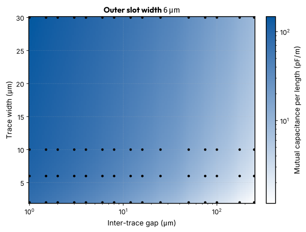
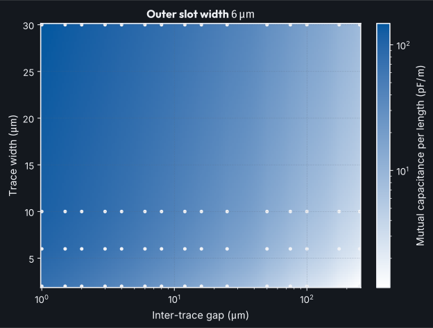
At a fixed outer slot width, vary trace width and inter-trace gap together. The black dots mark solved geometries; colours between them are interpolation. The logarithmic colour scale resolves weak coupling at large separations.

width_axis = jnp.linspace(*cpw_lookup.domain["width"], 101)
gap_axis = jnp.geomspace(*cpw_lookup.domain["gap"], 151)
W, G = jnp.meshgrid(width_axis, gap_axis, indexing="ij")
mutual_per_length = -cpw_lookup(width=W, cpw_gap=6.0, gap=G)[..., 0, 1] / slice_length
fig, ax = plt.subplots(constrained_layout=True)
image = ax.pcolormesh(
    gap_axis,
    width_axis,
    mutual_per_length * 1e12,
    cmap=QPDK,
    norm=LogNorm(),
    shading="auto",
    rasterized=True,
)
solved_width, solved_gap = jnp.meshgrid(
    cpw_grid.coords[0], cpw_grid.coords[2], indexing="ij"
)
ax.scatter(solved_gap, solved_width, s=8, color="black")
ax.set_xlabel(r"Inter-trace gap ($\text{µm}$)")
ax.set_xscale("log")
ax.set_ylabel(r"Trace width ($\text{µm}$)")
ax.set_title(r"Outer slot width $6\,\text{µm}$")
fig.colorbar(image, ax=ax, label=r"Mutual capacitance per length ($\text{pF/m}$)")
plt.show()

../_images/b8f5237ebc25ad4f883bbf453bb055a14a4973ec9f83a424ab88b51d16da363c.svg

../_images/b8f5237ebc25ad4f883bbf453bb055a14a4973ec9f83a424ab88b51d16da363c_dark.svg

Slices through the three-dimensional lookup#

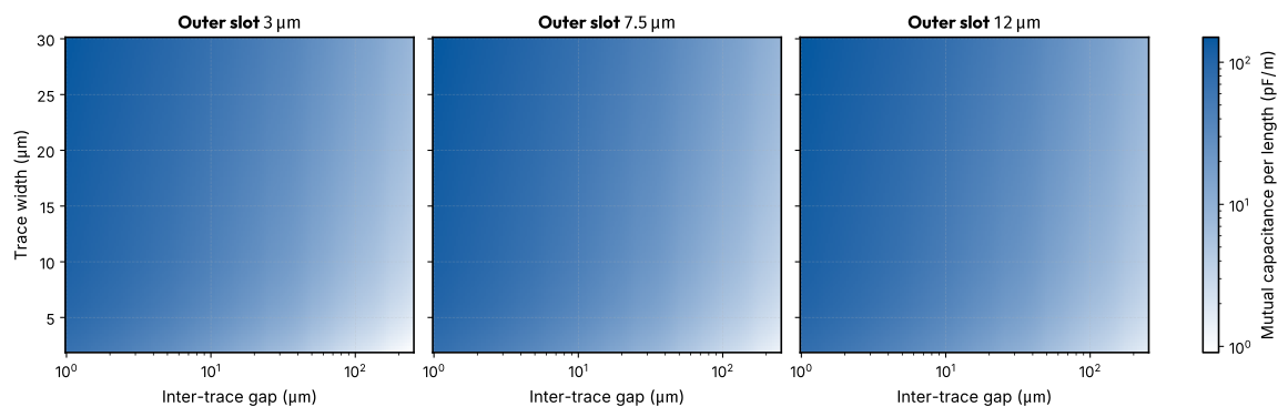
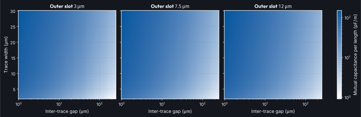
These three heatmaps vary all three parameters: the outer slot width changes between panels, while each panel scans trace width and inter-trace gap. A shared colour scale makes the effect of the third axis visible. The middle panel’s slot width lies between stored grid points.

outer_slots = jnp.array([3.0, 7.5, 12.0])
volume_slices = (
    -cpw_lookup(
        width=W[None, ...], cpw_gap=outer_slots[:, None, None], gap=G[None, ...]
    )[..., 0, 1]
    / slice_length
    * 1e12
)
fig, axes = plt.subplots(
    1, 3, figsize=(12, 3.8), sharex=True, sharey=True, constrained_layout=True
)
heatmap_norm = LogNorm(vmin=float(volume_slices.min()), vmax=float(volume_slices.max()))
for i, ax in enumerate(axes):
    image = ax.pcolormesh(
        gap_axis,
        width_axis,
        volume_slices[i],
        cmap=QPDK,
        norm=heatmap_norm,
        shading="auto",
        rasterized=True,
    )
    ax.set_title(rf"Outer slot ${float(outer_slots[i]):g}\,\text{{µm}}$")
    ax.set_xlabel(r"Inter-trace gap ($\text{µm}$)")
    ax.set_xscale("log")
axes[0].set_ylabel(r"Trace width ($\text{µm}$)")
fig.colorbar(
    image, ax=list(axes), label=r"Mutual capacitance per length ($\text{pF/m}$)"
)
plt.show()

../_images/1b92784469f3937d69fe72e40b10ae46ec8b30b82260a8bc31a80863a653bccf.svg

../_images/1b92784469f3937d69fe72e40b10ae46ec8b30b82260a8bc31a80863a653bccf_dark.svg

Compare with conformal mapping#

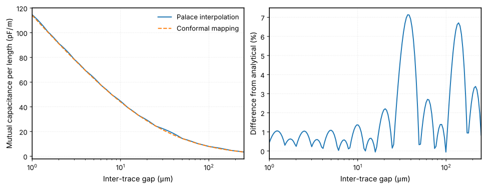
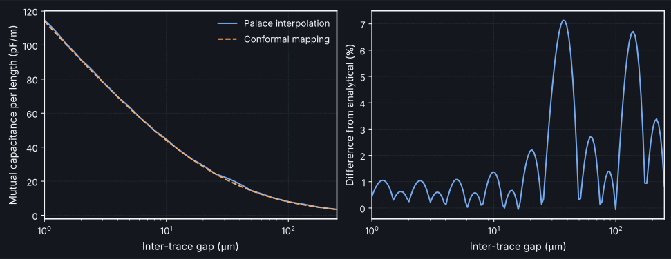
The analytical edge-coupled CPW expression assumes the same conductor sheets and dielectric half-spaces. Compare mutual capacitance per length directly, before turning either result into a circuit model.

analytical = cpw_cpw_coupling_capacitance_per_length_analytical(
    gap=gap_axis,
    width=10.0,
    cpw_gap=6.0,
    ep_r=cpw_dataset.metadata.provenance["settings"]["permittivity"],
)
fem = -cpw_lookup(width=10.0, cpw_gap=6.0, gap=gap_axis)[..., 0, 1] / slice_length
fig, axes = plt.subplots(1, 2, figsize=(10, 3.8), constrained_layout=True)
axes[0].plot(gap_axis, fem * 1e12, label="Palace interpolation")
axes[0].plot(gap_axis, analytical * 1e12, "--", label="Conformal mapping")
axes[0].set_ylabel(r"Mutual capacitance per length ($\text{pF/m}$)")
axes[0].legend()
axes[1].plot(gap_axis, 100 * (fem / analytical - 1))
axes[1].set_ylabel(r"Difference from analytical ($\text{%}$)")
for ax in axes:
    ax.set_xlabel(r"Inter-trace gap ($\text{µm}$)")
    ax.set_xscale("log")
plt.show()

../_images/ca55fe2d7774dbaa146a80e72a2f3f4b2084ee2002fe359e1f20e9a34bbac0cb.svg

../_images/ca55fe2d7774dbaa146a80e72a2f3f4b2084ee2002fe359e1f20e9a34bbac0cb_dark.svg

Ground left between the CPW slots#

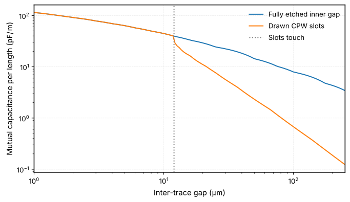
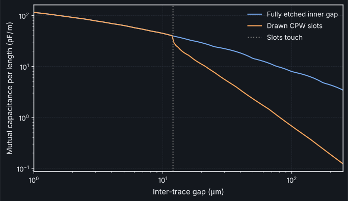
coupler_straight etches a slot on each side of each trace. When the inter-trace gap exceeds twice the slot width, a ground strip remains between the slots. The as-drawn experiment keeps this strip at reference ground. It matches the fully etched geometry while the slots touch or overlap; beyond that point, the ground shields the traces. The FEM capacitances are solved independently; the analytical expression is used only for comparison. Both models share ideal sheets and dielectric half-spaces. The analytical ECCPW formula assumes a fully etched inner gap, so its difference from the shielded result measures a geometry change as well as numerical error. Positive strip widths are sampled logarithmically from 0.01 µm. Logarithmic interpolation follows the rapid shielding onset; narrower strips return NaN.

layout_dataset = Dataset("cpw_coupling_ground_strip_palace")
layout_mutual = cpw_cpw_coupling_capacitance(
    f=5e9,
    length=1e6,
    gap=gap_axis,
    cross_section=coplanar_waveguide(width=10.0, gap=6.0),
)
fig, ax = plt.subplots(figsize=(7, 4), constrained_layout=True)
ax.loglog(gap_axis, fem * 1e12, label="Fully etched inner gap")
ax.loglog(gap_axis, layout_mutual * 1e12, label="Drawn CPW slots")
ax.axvline(12.0, color="gray", linestyle=":", label="Slots touch")
ax.set_xlabel(r"Inter-trace gap ($\text{µm}$)")
ax.set_ylabel(r"Mutual capacitance per length ($\text{pF/m}$)")
ax.legend()
plt.show()

../_images/4c813c25ae32d073ef4280bd4c5d1185b33cebbd1ed74146d45d2a81cca33646.svg

../_images/4c813c25ae32d073ef4280bd4c5d1185b33cebbd1ed74146d45d2a81cca33646_dark.svg

Compare both lookups with reference solves refined to a 0.1% successive-mesh change, larger domains, vacuum scaling and independent held-out geometries. Vacuum scaling uses byte-identical meshes to separate material scaling from refinement choices. These finite checks estimate sensitivity; they do not prove a uniform error bound.

quality_rows = []
for label, data in (("Etched gap", cpw_dataset), ("Ground strip", layout_dataset)):
    checks = data.metadata.provenance["validation"]
    quality_rows.append({
        "Geometry": label,
        "Mesh (%)": 100 * checks["maximum_mesh_relative_change"],
        "Reference (%)": 100 * checks["representative_stricter_mesh_max_relative"],
        "Initial domain (%)": 100
        * max(
            c["original_domain_relative"]
            for c in checks["mesh_domain"]
            if "original_domain_relative" in c
        ),
        "Domain (%)": 100 * max(c["domain_relative"] for c in checks["mesh_domain"]),
        "Same-mesh vacuum (%)": 100
        * max(c["vacuum_scaling_relative"] for c in checks["mesh_domain"]),
        "Lookup (%)": 100 * checks["held_out_max_relative"],
    })
pl.DataFrame(quality_rows)

shape: (2, 7)

Geometry	Mesh (%)	Reference (%)	Initial domain (%)	Domain (%)	Same-mesh vacuum (%)	Lookup (%)
str	f64	f64	f64	f64	f64	f64
"Etched gap"	0.997168	0.347286	1.208178	0.317497	0.015447	4.069779
"Ground strip"	0.99997	0.78594	1.27112	0.173371	0.003599	4.478808

The widest gaps needed larger domains and finer meshes. Each correction records its raw solver source and the comparison with a separate finer reference.

pl.DataFrame([
    {
        "Geometry": label,
        "Width (µm)": report["point"]["width"],
        "Slot (µm)": report["point"]["cpw_gap"],
        "Inner span (µm)": report["point"][
            "gap" if label == "Etched gap" else "ground_strip_width"
        ],
        "Original pad (µm)": report["previous_domain_pad_um"],
        "Accepted pad (µm)": report["accepted_domain_pad_um"],
        "Original mesh": report["previous_refinement_level"],
        "Accepted mesh": report["accepted_refinement_level"],
        "Original/reference (%)": 100 * report["reference_max_relative_before"],
        "Accepted/reference (%)": 100 * report["reference_max_relative_after"],
    }
    for label, data in (("Etched gap", cpw_dataset), ("Ground strip", layout_dataset))
    for report in data.metadata.provenance["curated_refinements"]
])

shape: (2, 10)

Geometry	Width (µm)	Slot (µm)	Inner span (µm)	Original pad (µm)	Accepted pad (µm)	Original mesh	Accepted mesh	Original/reference (%)	Accepted/reference (%)
str	f64	f64	f64	f64	f64	i64	i64	f64	f64
"Etched gap"	30.0	20.0	250.0	1350.0	2700.0	1	5	0.686527	0.089547
"Ground strip"	30.0	20.0	248.0	2025.0	4050.0	1	7	0.84599	0.068249

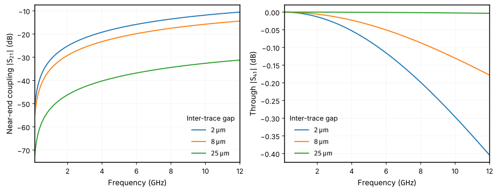
A distributed four-port SAX model#

cpw_cpw_coupling_capacitance() uses the layout-matching lookup in coupler_straight(). For a distributed section, cpw_coupling_model() loads and validates the grid once, then returns a jittable model of the uniform coupled section. The slice capacitances determine even- and odd-mode impedances. Geometric inductance follows the quasi-TEM dielectric half-space relation; kinetic inductance, finite substrate thickness, dispersion and loss are omitted.

Ports are o1 lower-left, o2 upper-left, o3 upper-right and o4 lower-right. Reference planes lie at the section ends. All four ports below use 50 ohm reference impedances. The remaining ports are matched when reading a single scattering entry; an open or short circuit must be connected explicitly in SAX.

cpw_model = cpw_coupling_model(layout_dataset)
frequencies = jnp.linspace(0.1e9, 12e9, 301)
fig, axes = plt.subplots(1, 2, figsize=(10, 3.8), constrained_layout=True)
for gap in (2.0, 8.0, 25.0):
    scattering = jax.jit(cpw_model)(
        f=frequencies, length=1000.0, width=10.0, cpw_gap=6.0, gap=gap
    )
    axes[0].plot(
        frequencies / 1e9,
        20 * jnp.log10(jnp.abs(scattering["o1", "o2"])),
        label=rf"${gap:g}\,\text{{µm}}$",
    )
    axes[1].plot(
        frequencies / 1e9,
        20 * jnp.log10(jnp.abs(scattering["o1", "o4"])),
        label=rf"${gap:g}\,\text{{µm}}$",
    )
axes[0].set_ylabel(r"Near-end coupling $|S_{21}|$ ($\text{dB}$)")
axes[1].set_ylabel(r"Through $|S_{41}|$ ($\text{dB}$)")
for ax in axes:
    ax.set_xlabel(r"Frequency ($\text{GHz}$)")
    ax.legend(title="Inter-trace gap")
plt.show()

../_images/e86492baa97a33c497251db8bf7e0b543cf0638411b28b416af4ed0302ee32b7.svg

../_images/e86492baa97a33c497251db8bf7e0b543cf0638411b28b416af4ed0302ee32b7_dark.svg

References#

[Jin14]

Jian-Ming Jin. The Finite Element Method in Electromagnetics. Wiley-IEEE Press, 3 edition, 2014. ISBN 978-1-118-57136-1.

[VD17]

Uri Vool and Michel Devoret. Introduction to quantum electromagnetic circuits. International Journal of Circuit Theory and Applications, 45(7):897–934, July 2017. doi:10.1002/cta.2359.

[WZ88]

Alan Weiser and Sergio E. Zarantonello. A note on piecewise linear and multilinear table interpolation in many dimensions. Mathematics of Computation, 50(181):189–196, 1988. doi:10.1090/S0025-5718-1988-0917826-0.