

Palace Flip-Chip Simulation of a Flipmon Qubit#
This notebook demonstrates a two-chip (flip-chip) FEM simulation of a flipmon: a circular transmon whose shunt capacitor is a vacuum-gap parallel-plate capacitor formed by flipping a second chip on top of the qubit chip [LZY+21]. It extends the Palace Eigenmode Simulation of a Transmon with a Readout Resonator notebook from a single chip to a two-chip stack: two metal levels, two sapphire substrates, and conducting indium bumps bridging the inter-chip gap, all driven through gsim and solved with Palace.
The flipmon topology, as drawn by flipmon_with_bbox():
The bottom chip (metal level M1) carries the inner circular pad, the outer ring, and the Josephson junction between them.
The top chip (metal level M2, flipped so its metal faces down) carries the top circle, galvanically connected to the inner pad through a central indium bump.
The qubit island is the inner pad + top circle node. The shunt capacitance is the vacuum gap between the top circle and the outer ring, which is the junction’s counter-electrode.
The workflow runs from layout to a qubit mode and its field:
        flowchart TB
    A["Flip-chip layout<br>(qpdk cells)"]
    B["FEM regions<br>(two metal levels + bumps)"]
    C["Two-chip layer stack"]
    D["Analytical estimate<br>(vacuum-gap capacitor)"]
    E["Mesh and eigenmode solve"]
    F["Compare with the paper<br>(frequency, capacitance, participation)"]
    A --> B --> C --> E --> F
    D --> F
Li et al. used a 5 µm gap, sapphire chips, tantalum electrodes, and indium bumps 20 to 50 µm across. Their simulated vacuum-gap electric-energy participation was 53.2% [LZY+21]. We use the reported gap and materials and a 30 µm bump. The paper does not specify the capacitor-pad radii or junction inductance, so those remain model choices.
Required extras
From a checkout, use Python 3.12 and install the palace dependency group:
uv sync --python 3.12 --extra models --group palace
The simulation cells additionally need the Palace solver itself, which is external to qpdk; the cells that invoke it are fenced, and the Palace results are embedded below so the analysis runs anywhere.
The standalone script and Colab setup also install the pinned gsim revision. See the extras reference for what each extra installs.
The results shown below were produced with Palace on an HPC cluster; the solver data is embedded in hidden cells so the rendered docs show the analysis, not the raw tables.
Simulation layout#
The device under test is the flipmon_with_bbox() cell: the
flipmon inside its etched bounding circles. The cell draws both metal levels
subtractively: each level’s etched bounding circle removes everything inside
it except the drawn pads, so the surrounding ground plane and the isolated
pads come out of the same mask.
Two additions make the standalone layout a well-posed simulation, and the wrapper below adds both:
Corner ground bumps. Four indium bumps tie the two ground planes together, as on the paper’s assembled chip.
Junction lead tabs. The lumped junction port must span the 20 µm gap between the inner circle and the outer ring as a rectangle. Both facing edges are circular arcs, so a rectangle clipped by them is no longer rectangular, and Palace rejects non-rectangular lumped port surfaces. Two small M1 lead tabs straighten the facing edges, narrowing the local lead gap to 12 µm the way real junction leads approach each other. The port rectangle must then exactly abut the tab edges: a port rectangle that overhangs the thin tabs makes the meshing pipeline’s boolean cuts delete them, which leaves the port electrically orphaned (verified below).
A SIM_AREA rectangle around the device bounds the simulation domain on
both chips.
BUMP_DIAMETER = 30.0  # µm, within the paper's reported 20 to 50 µm range
BUMP_RADIUS = BUMP_DIAMETER / 2


def _bump(x: float, y: float) -> kdb.DPolygon:
    """Return a circular bump polygon of the standard radius at (x, y)."""
    return kdb.DPolygon.ellipse(
        kdb.DBox(x - BUMP_RADIUS, y - BUMP_RADIUS, x + BUMP_RADIUS, y + BUMP_RADIUS), 64
    )


@gf.cell
def sim_component() -> gf.Component:
    """Flipmon with corner ground bumps, lead tabs and a simulation area."""
    c = gf.Component()
    ref = c << flipmon_with_bbox(bump_diameter=BUMP_DIAMETER)
    c.add_ports(ref.ports)
    # Tie the two chips' ground planes into a single ground node.
    for x, y in ((-150, -150), (150, -150), (-150, 150), (150, 150)):
        c.kdb_cell.shapes(gf.get_layer(LAYER.IND)).insert(_bump(x, y))
    # Junction lead tabs: straight metal edges across the junction gap so the
    # lumped port spans a rectangular lead gap instead of curved circle arcs.
    half_width = ref.ports["junction"].width / 2
    c.kdb_cell.shapes(gf.get_layer(LAYER.M1_DRAW)).insert(
        kdb.DBox(52.0, -half_width, 60.0, half_width)
    )
    c.kdb_cell.shapes(gf.get_layer(LAYER.M1_DRAW)).insert(
        kdb.DBox(72.0, -half_width, 80.0, half_width)
    )
    c.kdb_cell.shapes(gf.get_layer(LAYER.SIM_AREA)).insert(c.bbox().enlarged(100, 100))
    return c


layout_c = sim_component()
logger.info(f"simulation area: {layout_c.bbox()}")
for port in layout_c.ports:
    logger.info(
        f"port {port.name}: ({port.center[0]:.1f}, {port.center[1]:.1f}) µm,"
        f" orientation {port.orientation:.0f}°"
    )
2026-10-28 11:53:30.660 | INFO | __main__:<module>:35 - simulation area: (-270,-270;270,270)
2026-10-28 11:53:30.660 | INFO | __main__:<module>:37 - port center: (0.0, 0.0) µm, orientation 0°
2026-10-28 11:53:30.660 | INFO | __main__:<module>:37 - port inner_ring_near_junction: (30.0, 0.0) µm, orientation 0°
2026-10-28 11:53:30.660 | INFO | __main__:<module>:37 - port outer_ring_near_junction: (80.0, 0.0) µm, orientation 180°
2026-10-28 11:53:30.661 | INFO | __main__:<module>:37 - port outer_ring_outside: (140.0, 0.0) µm, orientation 0°
2026-10-28 11:53:30.661 | INFO | __main__:<module>:37 - port junction: (67.4, 0.0) µm, orientation 90°
From etch layers to flip-chip regions#
to_flip_chip_regions() applies the subtractive
convention on both metal levels (conductor is SIM_AREA - ETCH + DRAW,
matching the flip-chip layer stack) and copies the indium bump layer to its
own region. The result carries six regions: two sapphire substrates, the two
zero-thickness metal sheets, the vacuum gap, and the bumps.
regions = to_flip_chip_regions(layout_c)
rlayout = regions.kdb_cell.layout()
for name, (lnum, ldt) in FLIP_CHIP_FEM_LAYERS.items():
    region = kdb.Region(regions.kdb_cell.begin_shapes_rec(rlayout.layer(lnum, ldt)))
    logger.info(
        f"{name:>14} ({lnum},{ldt}): {len(region.merged())} polygons,"
        f" {region.area() / 1e6:.0f} µm²"
    )
2026-10-28 11:53:30.665 | INFO | __main__:<module>:5 - SUBSTRATE (114,0): 1 polygons, 291600 µm²
2026-10-28 11:53:30.665 | INFO | __main__:<module>:5 - M1 (115,0): 3 polygons, 253965 µm²
2026-10-28 11:53:30.665 | INFO | __main__:<module>:5 - VACUUM (116,0): 1 polygons, 291600 µm²
2026-10-28 11:53:30.666 | INFO | __main__:<module>:5 - BUMP (117,0): 5 polygons, 3530 µm²
2026-10-28 11:53:30.666 | INFO | __main__:<module>:5 - M2 (118,0): 2 polygons, 258938 µm²
2026-10-28 11:53:30.666 | INFO | __main__:<module>:5 - SUBSTRATE_TOP (119,0): 1 polygons, 291600 µm²
The region counts are the circuit topology made visible. M1 splits into the ground plane, the isolated outer ring and the isolated inner circle; M2 into the top ground plane and the isolated top circle. Each of the five bumps overlaps conductor on both chips, so they connect what they must connect: the one at the center joins the inner circle to the top circle (the qubit island); the four at the corners join the ground planes.
m1 = kdb.Region(
    regions.kdb_cell.begin_shapes_rec(rlayout.layer(*FLIP_CHIP_FEM_LAYERS["M1"]))
).merged()
m2 = kdb.Region(
    regions.kdb_cell.begin_shapes_rec(rlayout.layer(*FLIP_CHIP_FEM_LAYERS["M2"]))
).merged()
bumps = kdb.Region(
    regions.kdb_cell.begin_shapes_rec(rlayout.layer(*FLIP_CHIP_FEM_LAYERS["BUMP"]))
).merged()
assert (bumps - m1).is_empty(), "a bump does not land on the bottom-chip metal"
assert (bumps - m2).is_empty(), "a bump does not land on the top-chip metal"
The same subtractive-to-positive conversion as the single-chip case, applied once per metal level; see From etch layers to simulation regions for the rule and Palace Eigenmode Simulation of a Transmon with a Readout Resonator for the walkthrough.
Analytical qubit estimate#
The vacuum-gap capacitor gives a first estimate of the qubit frequency before any mesh is built. Treat the top circle and the outer ring as parallel plates across the inter-chip gap \(g\); the overlapping area is the annulus between the ring’s inner edge (radius 80 µm) and the top circle’s edge (radius 110 µm):
The qubit island also sees fringing fields at the plate edges, the substrate beneath both chips, and the small M1-level capacitance across the junction gap, so \(C_\Sigma > C_\text{vac}\) and the parallel-plate value bounds the qubit frequency from above. Deep in the transmon regime the linearized mode sits at \(f_q \approx 1 / (2\pi\sqrt{L_\text{J} C_\Sigma})\) [KYG+07, KKY+19].
BUMP_THICKNESS = 5.0  # µm, paper's nominal inter-chip gap
TOP_CIRCLE_RADIUS = 110.0  # µm
RING_INNER_RADIUS = 80.0  # µm
L_J = 8e-9  # H, linearized junction inductance

c_vac = (
    ε_0
    * jnp.pi
    * (TOP_CIRCLE_RADIUS**2 - RING_INNER_RADIUS**2)
    * 1e-12
    / (BUMP_THICKNESS * 1e-6)
)
f_q_upper = 1 / (2 * jnp.pi * jnp.sqrt(L_J * c_vac))
logger.info(f"parallel-plate vacuum capacitance: {c_vac * 1e15:.2f} fF")
logger.info(f"qubit frequency upper bound: {f_q_upper / 1e9:.2f} GHz")
2026-10-28 11:53:30.695 | INFO | __main__:<module>:14 - parallel-plate vacuum capacitance: 31.71 fF
2026-10-28 11:53:30.703 | INFO | __main__:<module>:15 - qubit frequency upper bound: 9.99 GHz
Simulation setup with gsim#
gsim turns the converted layout into a 3-D model: flip_chip_stack assigns
each region a material and a z-extent, and the simulation classes configure
the ports. The palace dependency group installs the pinned gsim version;
only the Palace solver itself stays external. The same geometry and stack
feed the saved eigenmode solve below.
The 5 µm vacuum gap and sapphire substrates follow the paper. We retain 500 µm substrate thickness as a model assumption; the paper does not give the wafer thickness. Gsim’s sapphire microwave permittivity is anisotropic (9.3 in-plane, 11.5 out-of-plane). The paper’s 120 nm tantalum films are represented as zero-thickness PEC sheets, while the indium bumps bridge the two metal levels as conductive vias.
The junction port points radially across the lead gap; resistance=0.0
keeps the linearized junction purely reactive.
from gsim.common.stack.materials import MATERIALS_DB

from qpdk.simulation import flip_chip_stack

stack = flip_chip_stack(substrate_thickness=500.0, bump_thickness=BUMP_THICKNESS)
for name in ("SUBSTRATE", "SUBSTRATE_TOP"):
    stack.layers[name].material = "sapphire"
stack.materials["sapphire"] = MATERIALS_DB["sapphire"].to_dict()
regions.ports["junction"].orientation = 0.0
# Center the port exactly on the 12 um lead gap (x from 60 to 72) so the
# port rectangle abuts both tab edges instead of overhanging them.
regions.ports["junction"].center = (66.0, 0.0)
pyvirtualdisplay not available; continuing without Xvfb
Mesh checks#
Gsim validates the mesh groups and Palace’s rectangular port geometry.
import json

from gsim.palace import EigenmodeSim, resolve_physical_groups

sim = EigenmodeSim()
sim.set_geometry(regions)
sim.set_stack(stack)
sim.set_numerical(order=1, solver_type="MUMPS")
# Exactly abut the 12 um lead gap: center the port on the gap and size the
# rectangle to it. An overhanging rectangle makes the boolean pipeline eat
# the lead tabs and orphan the port (see the port connectivity check).
sim.add_port("junction", layer="M1", length=12.0, inductance=L_J, resistance=0.0)
sim.set_eigenmode(target=4.8e9, num_modes=1, save=1)

SIM_DIR = Path("build/sim_palace_flipmon")
sim.set_output_dir(SIM_DIR)
if os.environ.get("QPDK_BUILD_FLIPMON") == "1":
    sim.mesh(preset="coarse", refined_mesh_size=0.5, auto_size=False)
    sim.write_config()
    sim.print_mesh_stats()
    sim.validate_mesh()
    config_path = SIM_DIR / "config.json"
    linear_config = json.loads(config_path.read_text())
    linear_config["Solver"]["Linear"]["MaxIts"] = 10
    linear_config["Solver"]["Linear"]["ColumnOrdering"] = "ParMETIS"
    linear_config["Solver"]["Eigenmode"]["Tol"] = 1e-3
    linear_config["Domains"]["Postprocessing"]["Energy"] = [
        {"Index": index, "Attributes": resolve_physical_groups(SIM_DIR, [name])}
        for index, name in enumerate(("VACUUM", "SUBSTRATE", "SUBSTRATE_TOP"), 1)
    ]
    config_path.write_text(json.dumps(linear_config, indent=2) + "\n")
/var/folders/7r/_fj6b8190zv3fsq1n4k2g0rh0000gn/T/ipykernel_44332/4037658474.py:8: DeprecationWarning: set_numerical() is deprecated; use set_solver() instead.
  sim.set_numerical(order=1, solver_type="MUMPS")
Simulation-area mesh#
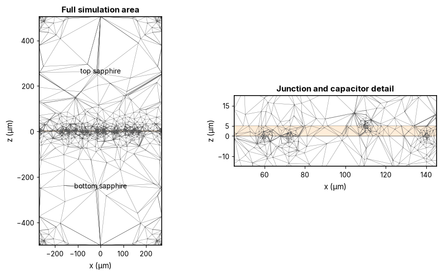
These views cut the tetrahedral grid saved with the Palace eigenmode at \(y=0\). The full section shows both 500 µm sapphire substrates and the simulation boundary. The detail resolves the 5 µm inter-chip gap and the junction leads. Both axes use the same physical scale within each panel. The mesh and fields below come from the same saved solution.
field_path = SIM_DIR / "output/palace/paraview/eigenmode/Cycle000001/data.pvtu"
field = None
if field_path.exists():
    import pyvista as pv

    field = pv.read(field_path)
    assert isinstance(field, pv.DataSet)
    section = field.slice(normal=(0, 1, 0), origin=(0, 0, BUMP_THICKNESS / 2))
    section = section.triangulate()
    assert isinstance(section, pv.PolyData)
    triangles = section.faces.reshape(-1, 4)[:, 1:]
    fig, axes = plt.subplots(1, 2, figsize=(9, 5.5), constrained_layout=True)
    for ax, limits, title in zip(
        axes,
        [
            ((field.bounds[0], field.bounds[1]), (field.bounds[4], field.bounds[5])),
            ((45, 145), (-15, 20)),
        ],
        ["Full simulation area", "Junction and capacitor detail"],
        strict=True,
    ):
        ax.axhspan(0, BUMP_THICKNESS, color="darkorange", alpha=0.15)
        ax.triplot(
            section.points[:, 0],
            section.points[:, 2],
            triangles,
            color="0.35",
            linewidth=0.3,
        )
        ax.set(xlim=limits[0], ylim=limits[1], xlabel="x (µm)", ylabel="z (µm)")
        ax.set_title(title)
        ax.set_aspect("equal")
        ax.grid(False)
    axes[0].text(0, -250, "bottom sapphire", ha="center")
    axes[0].text(0, 255, "top sapphire", ha="center")
    axes[1].set_yticks([-10, 0, 5, 15])
    plt.show()
    plt.close(fig)
else:
    logger.info("Palace field files are needed to regenerate the mesh sections")
findfont: Failed to find font weight bold, now using 400.
Solved qubit mode#
Palace identifies mode 1 by its junction inductive-energy participation. These values are from the saved first-order, 0.5 µm near-metal solve. Domain electric energies come from the same eigenmode; the vacuum domain is the 5 µm gap between the chips.
2026-10-28 11:53:31.966 | INFO | __main__:<module>:7 - mode 1: 4.9922 GHz, junction participation 0.9986, vacuum-gap electric participation 42.1%
2026-10-28 11:53:31.966 | INFO | __main__:<module>:12 - 0.70 to 0.50 µm mesh shift: 8.6 MHz
Comparison with Li et al.#
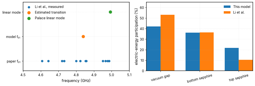
The Palace frequency is the linearized LC mode. We estimate the transmon transition by subtracting \(E_\text{C}/h\), with \(E_\text{C}=e^2/(2C_\Sigma)\) and \(C_\Sigma=[(2\pi f_\text{lin})^2 L_\text{J}]^{-1}\). The subtraction is a scale check, not a fitted junction model.
f_q = float(eig_f_ghz[0])
c_sigma = 1 / (2 * jnp.pi * f_q * 1e9) ** 2 / L_J
charging_ghz = e**2 / (2 * h * c_sigma) / 1e9
estimated_transition_ghz = f_q - charging_ghz
paper_fq_ghz = np.array([
    4.800,
    4.853,
    4.642,
    4.823,
    4.720,
    4.608,
    4.965,
    4.732,
    4.986,
    4.978,
    4.857,
    4.951,
])
logger.info(
    f"C_sigma = {c_sigma * 1e15:.1f} fF, E_C/h = {charging_ghz * 1e3:.0f} MHz, "
    f"estimated f_01 = {estimated_transition_ghz:.3f} GHz"
)

fig, axes = plt.subplots(1, 2, figsize=(10.5, 3.5), constrained_layout=True)
axes[0].scatter(paper_fq_ghz, np.zeros_like(paper_fq_ghz), label="Li et al., measured")
axes[0].scatter([estimated_transition_ghz], [1], s=75, label="Estimated transition")
axes[0].scatter([f_q], [2], s=75, label="Palace linear mode")
axes[0].set_yticks([0, 1, 2], [r"paper $f_{01}$", r"model $f_{01}$", "linear mode"])
axes[0].set_xlim(4.5, 5.1)
axes[0].set_ylim(-0.4, 2.4)
axes[0].set_xlabel("frequency (GHz)")
axes[0].legend(loc="upper left")
positions = np.arange(3)
axes[1].bar(positions - 0.18, electric_epr * 100, width=0.36, label="This model")
axes[1].bar(positions + 0.18, paper_electric_epr * 100, width=0.36, label="Li et al.")
axes[1].set_xticks(positions, ["vacuum gap", "bottom sapphire", "top sapphire"])
axes[1].set_ylabel("electric-energy participation (%)")
axes[1].set_ylim(0, 65)
axes[1].tick_params(axis="x", labelrotation=15)
axes[1].legend()
plt.show()
plt.close(fig)
2026-10-28 11:53:31.970 | INFO | __main__:<module>:19 - C_sigma = 127.0 fF, E_C/h = 152 MHz, estimated f_01 = 4.840 GHz
Quantity |
Li et al. |
This model |
|---|---|---|
Chip gap |
\(5\pm0.4\,\text{µm}\) measured |
\(5\,\text{µm}\) |
Substrates |
Sapphire |
Sapphire |
Indium bump diameter |
\(20\) to \(50\,\text{µm}\) |
\(30\,\text{µm}\) |
Qubit \(f_{01}\) |
\(4.608\) to \(4.986\,\text{GHz}\) measured |
\(4.840\,\text{GHz}\) estimated from a \(4.992\,\text{GHz}\) linear mode |
\(C_\Sigma\) |
\(78\) to \(88\,\text{fF}\) inferred from anharmonicity |
\(127.0\,\text{fF}\) inferred with \(L_\text{J}=8\,\text{nH}\) |
Vacuum-gap electric-energy participation |
\(53.2\%\) simulated |
\(42.1\%\) simulated |
Bottom-sapphire electric-energy participation |
\(36.3\%\) simulated |
\(36.1\%\) simulated |
Top-sapphire electric-energy participation |
\(10.5\%\) simulated |
\(21.8\%\) simulated |
The gap, substrate, and bump size follow the paper. Its pad radii and junction inductance are not specified. The bottom-sapphire share agrees, while the model has less energy in the gap and more in the top substrate. The raw eigenmode \(Q\) uses the stack’s bulk sapphire loss and does not predict the measured \(T_1\). The inductive junction participation and electric vacuum participation are different quantities.
Electric field in the gap#
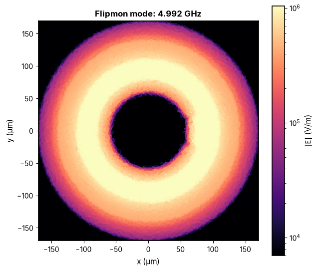
The saved image samples Palace’s mode-1 field halfway across the vacuum gap, at \(z=2.5\,\text{µm}\). Palace exports electric field values local to each mesh element; a planar cut can therefore show small facets. Sampling onto a regular grid and filtering over 0.4 µm reduces those seams without changing the solved field. The PNG is embedded in the notebook output.
if field is not None:
    import pyvista as pv

    x = np.linspace(-170, 170, 850)
    y = np.linspace(-170, 170, 850)
    grid_x, grid_y = np.meshgrid(x, y)
    points = np.column_stack((
        grid_x.ravel(),
        grid_y.ravel(),
        np.full(grid_x.size, 2.5),
    ))
    sampled = pv.PolyData(points).sample(field)
    valid = np.asarray(sampled.point_data["vtkValidPointMask"], dtype=bool).reshape(
        grid_x.shape
    )
    e_real = np.asarray(sampled.point_data["E_real"], dtype=float)
    e_imag = np.asarray(sampled.point_data["E_imag"], dtype=float)
    magnitude = np.sqrt(np.sum(e_real**2 + e_imag**2, axis=1)).reshape(grid_x.shape)
    positive = magnitude[valid & (magnitude > 0)]
    vmax = float(np.percentile(positive, 99.5))
    vmin = max(vmax / 150, float(np.percentile(positive, 25)))
    sigma = 0.4 / (x[1] - x[0])
    weights = valid.astype(float)
    log_field = np.log(np.where(valid, np.maximum(magnitude, vmin), vmin))
    shown = np.where(
        valid,
        np.exp(
            gaussian_filter(log_field * weights, sigma)
            / np.maximum(gaussian_filter(weights, sigma), 1e-12)
        ),
        np.nan,
    )
    cmap = plt.get_cmap("magma").copy()
    cmap.set_bad("0.94")
    fig, ax = plt.subplots(figsize=(6.5, 5.7))
    image = ax.imshow(
        shown,
        origin="lower",
        extent=(-170, 170, -170, 170),
        cmap=cmap,
        norm=LogNorm(vmin=vmin, vmax=vmax),
        interpolation="none",
    )
    ax.grid(False)
    ax.set_aspect("equal")
    ax.set_xlabel("x (µm)")
    ax.set_ylabel("y (µm)")
    ax.set_title(f"Flipmon mode: {f_q:.3f} GHz")
    fig.colorbar(image, ax=ax, label=r"$|\mathbf{E}|$ (V/m)")
    plt.show()
    plt.close(fig)
else:
    logger.info("Palace field files are needed to regenerate the embedded plot")
Vertical electric-field section#
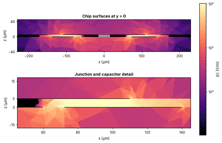
The \(y=0\) section shows the field across both chip surfaces. The lower panel zooms in on the junction and the overlap between the outer ring and top pad. Black lines are the actual metal intersections, and gray marks the central indium bump. The bottom metal is at \(z=0\) and the top metal at \(z=5\,\text{µm}\).
These samples are unsmoothed so the normal-field jump between sapphire and vacuum remains visible. Both panels share one color scale. Eigenmode field amplitudes have arbitrary normalization, not a specified drive voltage.
if field is not None:
    import pyvista as pv

    x = np.linspace(-230, 230, 1151)
    # Avoid sampling exactly on the zero-thickness metal planes.
    z = np.arange(-400, 451) * 0.1 + 0.025
    grid_x, grid_z = np.meshgrid(x, z)
    points = np.column_stack((grid_x.ravel(), np.zeros(grid_x.size), grid_z.ravel()))
    sampled = pv.PolyData(points).sample(field)
    valid = np.asarray(sampled.point_data["vtkValidPointMask"], dtype=bool).reshape(
        grid_x.shape
    )
    e_real = np.asarray(sampled.point_data["E_real"], dtype=float)
    e_imag = np.asarray(sampled.point_data["E_imag"], dtype=float)
    magnitude = np.sqrt(np.sum(e_real**2 + e_imag**2, axis=1)).reshape(grid_x.shape)
    positive = magnitude[valid & (magnitude > 0)]
    vmax = float(np.percentile(positive, 99.5))
    norm = LogNorm(vmin=vmax / 1000, vmax=vmax)
    cut = kdb.Region(kdb.DBox(-270, -0.001, 270, 0.001).to_itype(regions.kcl.dbu))
    cmap = plt.get_cmap("magma").copy()
    cmap.set_bad("0.94")
    fig, axes = plt.subplots(2, 1, figsize=(9, 5.8), constrained_layout=True)
    for ax, limits, title in zip(
        axes,
        [((-230, 230), (-40, 45)), ((45, 145), (-12, 17))],
        ["Chip surfaces at y = 0", "Junction and capacitor detail"],
        strict=True,
    ):
        ax.pcolormesh(
            x,
            z,
            np.ma.array(magnitude, mask=~valid),
            cmap=cmap,
            norm=norm,
            shading="nearest",
            rasterized=True,
        )
        for metal, height in ((m1, 0), (m2, BUMP_THICKNESS)):
            for polygon in metal & cut:
                bounds = polygon.to_dtype(regions.kcl.dbu).bbox()
                ax.hlines(
                    height, bounds.left, bounds.right, color="black", linewidth=1.2
                )
        for polygon in bumps & cut:
            bounds = polygon.to_dtype(regions.kcl.dbu).bbox()
            ax.fill_between(
                [bounds.left, bounds.right], 0, BUMP_THICKNESS, color="0.6", zorder=3
            )
        ax.set(xlim=limits[0], ylim=limits[1], xlabel="x (µm)", ylabel="z (µm)")
        ax.set_title(title)
        ax.set_aspect("equal")
        ax.grid(False)
    axes[0].set_yticks([-40, 0, 40])
    axes[1].set_yticks([-10, 0, 5, 15])
    fig.colorbar(
        plt.cm.ScalarMappable(norm=norm, cmap=cmap),
        ax=axes,
        label=r"$|\mathbf{E}|$ (V/m)",
    )
    plt.show()
    plt.close(fig)
else:
    logger.info("Palace field files are needed to regenerate the vertical section")
Summary#
The 5 µm sapphire stack produces a junction mode near the paper’s measured band. The 0.70 to 0.50 µm mesh change moves its linear frequency by 8.6 MHz. Its vacuum-gap participation is lower than the paper’s FEM value, which is useful evidence that the unspecified pad geometry still matters.
The mesh sections, field slices and participation plot use the saved Palace solution. A surface-loss model and a device-specific junction are needed to compare lifetimes.
References#
Jens Koch, Terri M. Yu, Jay Gambetta, A. A. Houck, D. I. Schuster, J. Majer, Alexandre Blais, M. H. Devoret, S. M. Girvin, and R. J. Schoelkopf. Charge-insensitive qubit design derived from the Cooper pair box. Physical Review A, 76(4):042319, October 2007. doi:10.1103/PhysRevA.76.042319.
P. Krantz, M. Kjaergaard, F. Yan, T. P. Orlando, S. Gustavsson, and W. D. Oliver. A quantum engineer's guide to superconducting qubits. Applied Physics Reviews, 6(2):021318, June 2019. doi:10.1063/1.5089550.
Xuegang Li, Yingshan Zhang, Chuhong Yang, Zhiyuan Li, Junhua Wang, Tang Su, Mo Chen, Yongchao Li, Chengyao Li, Zhenyu Mi, Xuehui Liang, Chenlu Wang, Zhen Yang, Yulong Feng, Kehuan Linghu, Huikai Xu, Jiaxiu Han, Weiyang Liu, Peng Zhao, Teng Ma, Ruixia Wang, Jingning Zhang, Yu Song, Pei Liu, Ziting Wang, Zhaohua Yang, Guangming Xue, Yirong Jin, and Haifeng Yu. Vacuum-gap transmon qubits realized using flip-chip technology. Applied Physics Letters, 119(18):184003, November 2021. doi:10.1063/5.0068255.