

Batched Layout Optimisation of a Transmon with Optuna#
This notebook extends Palace Eigenmode Simulation of a Transmon with a Readout Resonator to a geometry sweep. Optuna proposes pad dimensions and gaps; Palace supplies the linearised qubit frequency and dielectric energy participation. The study keeps frequency error, quality factor, and pad area as separate Pareto objectives.
The dielectric loss model follows [Sav23]:
The electromagnetic mode needs an anharmonic correction to estimate the 0-1 transition. \(T_1\) is a derived check; its \(1/f\) factor would otherwise favour low frequencies even when the field loss is unchanged.
Required extras
Install models and optimization. The optional Ray backend also needs ray:
uv add "qpdk[models,optimization]"
# in this repository:
uv sync --extra models --extra optimization --group palace
# with pip:
pip install "qpdk[models,optimization]"
Palace is external to qpdk. Saved trial results let the analysis render without running the solver.
The standalone script and Colab setup also install the pinned gsim revision. See the extras reference for what each extra installs.
Note
The launcher shows how to repeat the study on Slurm.
import io
import json
import os
import shlex
import sys
from dataclasses import dataclass, replace
from pathlib import Path
from typing import Any, Literal

import matplotlib

# The same source file is the cluster driver, where there is no display and a
# blocking figure would hang the batch. Rendering inside a kernel keeps the
# interactive backend so the figures appear inline.
if "ipykernel" not in sys.modules:
    matplotlib.use("Agg")

import gdsfactory as gf
import klayout.db as kdb
import matplotlib.pyplot as plt
import numpy as np
import optuna
import pandas as pd
from matplotlib import font_manager

import qpdk.colormaps  # ruff: ignore[unused-import] - registers the style colormap
from qpdk import PDK, logger
from qpdk.cells import double_pad_transmon_with_bbox
from qpdk.config import PATH
from qpdk.logger import PLAIN_FORMAT, configure_logger
from qpdk.simulation import SlurmCluster
from qpdk.simulation.fem import FEM_LAYERS, single_chip_stack, to_fem_regions
from qpdk.simulation.palace_run import (
    add_domain_energy_postprocessing,
    domain_loss_tangents,
    solve,
    verify_port_connectivity,
)
from qpdk.simulation.study import RayRunner, SlurmRunner, run_study

PDK.activate()

for style in (PATH.repo / "docs" / "qpdk.mplstyle", "qpdk"):
    try:
        plt.style.use(style)
    except OSError:
        continue
    break

for font_path in (PATH.repo / "build" / "docs-fonts").glob("*"):
    if font_path.suffix.lower() in {".otf", ".ttf"}:
        font_manager.fontManager.addfont(str(font_path))

installed_fonts = {font.name for font in font_manager.fontManager.ttflist}
plt.rcParams["font.sans-serif"] = [
    name
    for name in ("Inter", "Outfit", "DejaVu Sans", "Helvetica", "Arial")
    if name in installed_fonts
] + ["sans-serif"]

if "ipykernel" in sys.modules:
    import matplotlib_inline

    # Raster outputs avoid Matplotlib SVG links that docs link checkers follow.
    matplotlib_inline.backend_inline.set_matplotlib_formats("png")
The device and its knobs#
The double_pad_transmon_with_bbox() cell has two pads and
a junction across their gap. We vary:
pad width, along the junction axis;
pad height, perpendicular to it;
pad gap, which the junction bridges.
The junction inductance stays fixed, so geometry changes the capacitance and the linearised frequency \(f_\text{lin}\approx 1/(2\pi\sqrt{L_\text{J}C_\Sigma})\).
PAD_WIDTH_RANGE = (80.0, 420.0)  # µm, along the junction gap
PAD_HEIGHT_RANGE = (150.0, 650.0)  # µm, perpendicular to it
PAD_GAP_RANGE = (10.0, 160.0)  # µm, island-island separation
LAYOUT_GRID_UM = 0.01

# A fixed inductor, so the geometry moves the linearised frequency through capacitance.
L_JUNCTION = 10e-9  # H
JUNCTION_PARTICIPATION_FLOOR = 0.5
F_TARGET = 4.5e9  # Hz, target linearised mode; the physical transition is lower
# How close to the target counts as on-target when picking a geometry.
TOLERANCE_BAND = 0.02
# Accept small Q differences when choosing a smaller pad footprint.
Q_SLACK = 0.01

# The study size follows the allocation rather than the other way round, so the
# Slurm launcher at the end of the notebook sets these from the job request.
# One switch for every cell that needs a solver, so a half-set value cannot
# run the demos and then silently skip the study.
RUN_OPTIMIZATION = os.environ.get("QPDK_RUN_OPTIMIZATION") == "1"
RUN_DEMO_SOLVE = os.environ.get("QPDK_RUN_DEMO_SOLVE") == "1"
if RUN_OPTIMIZATION:
    # The driver's stdout is a Slurm .out file someone will `tail -f`, not a
    # terminal, so drop the colour escapes and the decoration.
    configure_logger(log_format=PLAIN_FORMAT, colorize=False)
MAX_IN_FLIGHT = int(os.environ.get("QPDK_MAX_IN_FLIGHT") or 6)  # trials at once
N_TRIALS = int(os.environ.get("QPDK_N_TRIALS") or 150)  # total trials
From a layout to a simulation directory#
Each trial converts the etch masks into conductor and dielectric regions
with to_fem_regions(), applies
single_chip_stack(), and writes a Palace mesh and
config. The junction port is turned to face across the pad gap. The config
requests domain energies so the loss objective can be reconstructed.
The junction sheet is 2 µm wide and spans the snapped pad gap exactly. Overhanging sheets remove PEC coverage inside the pads during meshing, as shown in Palace Eigenmode Simulation of a Transmon with a Readout Resonator. The checks below reject overlap and require contact with both pad edges.
@dataclass(slots=True, frozen=True, kw_only=True)
class Layout:
    """One candidate double-pad transmon geometry.

    Attributes:
        pad_width: Pad extent along the junction gap, in µm.
        pad_height: Pad extent perpendicular to the gap, in µm.
        pad_gap: Island-island separation the junction bridges, in µm.
    """

    pad_width: float
    pad_height: float
    pad_gap: float

    @property
    def pad_size(self) -> tuple[float, float]:
        """Pad size in µm, as the cell expects it."""
        return (self.pad_width, self.pad_height)

    @property
    def footprint_mm2(self) -> float:
        """Metal area of the two pads in mm².

        The qubit's footprint, which is what a chip pays for in real estate and
        what stands in for the coupling and crosstalk a larger qubit invites.
        Only the pads are counted; the etch around them belongs to the ground
        plane and scales with the gap.
        """
        return 2.0 * self.pad_width * self.pad_height / 1e6


def transmon_sim_layout(
    pad_size: tuple[float, float], pad_gap: float, margin: float = 250.0
) -> gf.Component:
    """Transmon pads wrapped in the area the solver meshes.

    Args:
        pad_size: Pad width and height in µm, snapped to a 10 nm grid.
        pad_gap: Island-island gap in µm, snapped to the same grid.
        margin: Space around the etched box to the simulation boundary in µm.

    Returns:
        Component carrying the layout, its ports, and a ``SIM_AREA`` rectangle
        bounding the simulation domain.
    """
    # Resolve the layer at call time so the notebook evaluator can be sent to workers.
    from qpdk.tech import LAYER

    grid_factor = round(LAYOUT_GRID_UM * 1000)
    pad_size = (
        gf.snap.snap_to_grid(pad_size[0], grid_factor=grid_factor),
        gf.snap.snap_to_grid(pad_size[1], grid_factor=grid_factor),
    )
    pad_gap = gf.snap.snap_to_grid(pad_gap, grid_factor=round(LAYOUT_GRID_UM * 1000))

    c = gf.Component()
    ref = c << double_pad_transmon_with_bbox(pad_size=pad_size, pad_gap=pad_gap)
    junction = ref.ports["junction"]
    c.add_port(
        "junction",
        center=junction.center,
        width=2.0,
        orientation=junction.orientation,
        layer=junction.layer,
        port_type=junction.port_type,
    )
    c.add_ports(ref.ports.filter(regex=r"^(?!junction$)"))
    c.kdb_cell.shapes(gf.get_layer(LAYER.SIM_AREA)).insert(
        c.bbox().enlarged(margin, margin)
    )
    return c


def build_simulation(
    layout: Layout,
    sim_dir: Path,
    *,
    junction_inductance: float = L_JUNCTION,
    num_modes: int = 3,
    substrate_thickness: float = 500.0,
    vacuum_thickness: float = 500.0,
    lateral_margin: float = 250.0,
    refined_mesh_size: float = 0.35,
    linear_max_its: int = 40,
    mesh_preset: Literal["coarse", "default", "fine"] = "coarse",
) -> Path:
    """Write a self-contained Palace eigenmode directory for ``layout``.

    The result is ``config.json`` plus ``palace.msh``, which is everything a
    Palace binary needs, so the directory can be handed to a worker on another
    node without any further state.

    Args:
        layout: Candidate geometry.
        sim_dir: Directory to write into; created if missing.
        junction_inductance: Linearised junction inductance in H.
        num_modes: Number of eigenmodes to solve for.
        substrate_thickness: Silicon thickness in µm.
        vacuum_thickness: Air height above the chip in µm.
        lateral_margin: Distance from the etch-box edge to the outer boundary in µm.
        refined_mesh_size: Near-conductor mesh size in µm.
        linear_max_its: Maximum iterations for the Palace linear solve.
        mesh_preset: Gmsh mesh preset.

    Returns:
        The simulation directory.
    """
    from gsim.palace import EigenmodeSim, resolve_physical_groups

    from qpdk import PDK

    # Worker imports need the PDK active to resolve cell layers.
    PDK.activate()

    sim_dir.mkdir(parents=True, exist_ok=True)
    regions = to_fem_regions(
        transmon_sim_layout(layout.pad_size, layout.pad_gap, lateral_margin)
    )
    # The cell's junction marker is perpendicular to the pad-to-pad axis.
    regions.ports["junction"].orientation = 0.0
    port_length = regions.ports["right_pad_inner"].x - regions.ports["left_pad_inner"].x
    metal = kdb.Region(
        regions.kdb_cell.begin_shapes_rec(
            regions.kdb_cell.layout().layer(*FEM_LAYERS["SUPERCONDUCTOR"])
        )
    ).merged()
    junction_sheet = kdb.Region(
        kdb.DBox(-port_length / 2, -1.0, port_length / 2, 1.0).to_itype(regions.kcl.dbu)
    )
    assert (junction_sheet & metal).is_empty(), "junction sheet overlaps pad metal"
    assert len(metal.interacting(junction_sheet.sized(1))) == 2, (
        "junction sheet must touch both pad edges"
    )

    sim = EigenmodeSim()
    sim.set_geometry(regions)
    sim.set_stack(
        single_chip_stack(
            substrate_thickness=substrate_thickness,
            vacuum_thickness=vacuum_thickness,
        )
    )
    sim.set_numerical(order=2, solver_type="MUMPS")
    # Gsim's default 50 Ohm port would add loss to the linearised junction.
    sim.add_port(
        "junction",
        layer="SUPERCONDUCTOR",
        length=port_length,
        inductance=junction_inductance,
        resistance=0.0,
    )
    sim.set_eigenmode(target=1e9, num_modes=num_modes)
    sim.set_output_dir(sim_dir)
    sim.mesh(preset=mesh_preset, refined_mesh_size=refined_mesh_size, auto_size=False)
    sim.write_config()
    config_path = sim_dir / "config.json"
    config = json.loads(config_path.read_text())
    config["Solver"]["Linear"].update({
        "MaxIts": linear_max_its,
        "Tol": 1e-5,
        "MGMaxLevels": 2,
        "PCMatReal": False,
        "PCMatShifted": False,
        "ComplexCoarseSolve": True,
        "ColumnOrdering": "ParMETIS",
    })
    config["Solver"]["Eigenmode"]["Tol"] = 1e-5
    surfaces = (
        ("SA", "SUBSTRATE__VACUUM"),
        ("MS", "SUPERCONDUCTOR_pec"),
        ("MA", "SUPERCONDUCTOR_pec"),
    )
    config["Boundaries"]["Postprocessing"] = {
        "Dielectric": [
            {
                "Index": index,
                "Attributes": resolve_physical_groups(sim_dir, [group]),
                "Type": kind,
                "Thickness": 3e-9 / config["Model"]["L0"],
                "Permittivity": 10.0,
                "LossTan": 1e-3,
            }
            for index, (kind, group) in enumerate(surfaces, start=1)
        ]
    }
    config_path.write_text(json.dumps(config, indent=2))
    add_domain_energy_postprocessing(sim_dir)
    verify_port_connectivity(sim_dir)
    return sim_dir


def evaluate_simulation(sim_dir: Path) -> dict[str, Any]:
    """Extract the transmon mode and its dielectric loss from a Palace solve.

    ``f_linear`` is the LC mode, so a target for the physical 0-1 transition
    needs the anharmonic correction from the inferred capacitance.

    Args:
        sim_dir: Simulation directory Palace wrote its ``output/`` into.

    Returns:
        A row of results: ``f_linear`` in Hz, ``T1`` in seconds, dielectric
        ``quality_factor`` from domain participations, the raw
        ``eigenmode_quality_factor``, junction participation, and per-domain
        electric-energy participations.

    Raises:
        FileNotFoundError: If the solve produced no eigenmode table.
        ValueError: If no mode carries junction energy.
    """
    from gsim.palace.results import load_text_results

    output = sim_dir / "output" / "palace"
    eig_path = output / "eig.csv"
    if not eig_path.exists():
        msg = f"Palace produced no eig.csv in {output}; see {sim_dir}/run.log"
        raise FileNotFoundError(msg)

    tables = load_text_results(output).csv_tables

    def table(name: str) -> list[dict[str, str]]:
        return [
            {key.strip(): value for key, value in row.items()} for row in tables[name]
        ]

    eig = table("eig.csv")
    junction = table("port-EPR.csv")
    domains = table("domain-E.csv")

    if not len(eig) == len(junction) == len(domains):
        msg = (
            f"Palace tables disagree on mode count in {output}: "
            f"eig={len(eig)}, port-EPR={len(junction)}, domain-E={len(domains)}"
        )
        raise ValueError(msg)

    participations = np.array([abs(float(row["p[1]"])) for row in junction])
    frequencies = np.array([float(row["Re{f} (GHz)"]) for row in eig])

    # A higher harmonic can have more junction energy, so choose the lowest
    # participating mode above the floor that excludes packaging modes.
    candidates = np.flatnonzero(participations >= JUNCTION_PARTICIPATION_FLOOR)
    if candidates.size == 0:
        msg = (
            "no mode carries junction energy; the lumped port is probably not "
            "spanning the pad gap"
        )
        raise ValueError(msg)
    index = int(candidates[np.argmin(frequencies[candidates])])

    f_linear = float(eig[index]["Re{f} (GHz)"]) * 1e9
    loss_tangents = domain_loss_tangents(sim_dir)
    domain_participations = {
        int(key[len("p_elec[") : -1]): float(value)
        for key, value in domains[index].items()
        if key.startswith("p_elec[")
    }
    if domain_participations.keys() != loss_tangents.keys():
        msg = f"domain-E.csv is missing a configured dielectric domain in {output}"
        raise ValueError(msg)
    inverse_q = sum(
        participation * loss_tangents[domain]
        for domain, participation in domain_participations.items()
    )
    quality_factor = 1.0 / inverse_q if inverse_q > 0 else float("inf")

    row: dict[str, Any] = {
        "f_linear": f_linear,
        "quality_factor": quality_factor,
        "eigenmode_quality_factor": float(eig[index]["Q"]),
        "T1": quality_factor / (2.0 * np.pi * f_linear),
        "junction_participation": float(participations[index]),
        "num_modes": len(eig),
        "mode_index": index + 1,
    }
    for domain, participation in domain_participations.items():
        row[f"participation_domain{domain}"] = participation
    if "surface-Q.csv" in tables:
        surfaces = table("surface-Q.csv")
        if len(surfaces) != len(eig):
            msg = f"surface-Q.csv disagrees on mode count in {output}"
            raise ValueError(msg)
        for surface_index, kind in enumerate(("sa", "ms", "ma"), start=1):
            row[f"participation_{kind}"] = float(
                surfaces[index][f"p_surf[{surface_index}]"]
            )
    return row


def trial_dir_name(layout: Layout) -> str:
    """Return the directory name a trial of ``layout`` is written under.

    Full float precision keeps distinct inputs distinct even when a serial
    caller passes values off the sampling grid.

    Args:
        layout: Candidate geometry.

    Returns:
        A directory name unique to these geometry values.
    """
    return f"w{layout.pad_width:.17g}_h{layout.pad_height:.17g}_g{layout.pad_gap:.17g}"


def evaluate_layout(
    params: dict[str, float],
    run_root: str | Path,
    *,
    ranks: int = 2,
    sim_dir: str | Path | None = None,
    timeout: float = 6000.0,
    **build_settings: Any,
) -> dict[str, Any]:
    """Build, solve and post-process one candidate geometry.

    This is the unit of work a sweep repeats, so it takes and returns plain
    data: everything it learns is either in the return value or on disk under
    ``run_root``, and a caller that dies loses only its own trial.

    Args:
        params: Keyword arguments for :class:`Layout`.
        run_root: Parent directory for trial output.
        ranks: MPI ranks to give each solve.
        sim_dir: Directory for this trial. Defaults to a geometry-named
            directory under ``run_root``, which is only safe when trials do not
            run concurrently.
        timeout: Seconds before a solve is abandoned. Size it under the trial
            job's wall clock, or Slurm kills the task first and the trial
            reports nothing.
        **build_settings: Forwarded to :func:`build_simulation`.

    Returns:
        The row from :func:`evaluate_simulation`, plus the geometry parameters.
    """
    layout = Layout(**params)
    # Geometry-named output is safe only when callers run serially.
    sim_dir = Path(sim_dir) if sim_dir else Path(run_root) / trial_dir_name(layout)
    build_settings.setdefault("junction_inductance", L_JUNCTION)
    build_simulation(layout, sim_dir, **build_settings)
    solve(sim_dir, ranks=ranks, timeout=timeout)
    return (
        evaluate_simulation(sim_dir) | params | {"footprint_mm2": layout.footprint_mm2}
    )
demo_layout = Layout(pad_width=250.0, pad_height=400.0, pad_gap=15.0)
demo_dir = Path("build/palace_optimization_demo")
# Meshing needs Gmsh and a large allocation, so the demo runs separately from
# the one-core sweep driver.
if RUN_DEMO_SOLVE:
    build_simulation(demo_layout, demo_dir)
    logger.info(f"wrote {demo_dir}")
Running Palace#
solve() launches Palace with MPI. Each
trial can use several nodes.
Reading a solve back into physics#
The evaluator reads eig.csv for frequency, port-EPR.csv to identify
the lowest junction-coupled mode, and domain-E.csv for dielectric energy.
It calculates the loss objective from those energies and the stack’s loss
tangents. The raw eigenfrequency \(Q\) remains a solver diagnostic.
# Run the demo inside an allocation sized like one trial before launching a sweep.
demo_result: dict[str, float] | None = None
if RUN_DEMO_SOLVE:
    solve(demo_dir, ranks=int(os.environ.get("QPDK_SOLVER_CORES") or 24))
    demo_result = evaluate_simulation(demo_dir)
    logger.info(
        f"demo layout: f_lin = {demo_result['f_linear'] / 1e9:.4f} GHz, "
        f"T1 = {demo_result['T1'] * 1e6:.2f} µs, "
        f"Q = {demo_result['quality_factor']:.3e}"
    )
Loss model#
Vacuum is lossless in this model. Silicon has the PDK loss tangent, so the reported \(Q_\text{diel}\) is limited by bulk silicon. Nanometre scale metal-air, metal-substrate, and substrate-air layers add loss in a fabricated device [Sav23]. Their participations are examined separately below; no interface loss tangent is assumed for the Pareto objective.
if demo_result is not None:
    tangents = domain_loss_tangents(demo_dir)
    budget = sum(
        demo_result[f"participation_domain{index}"] * tangent
        for index, tangent in tangents.items()
    )
    logger.info(
        f"1/Q from participations {budget:.4e}; "
        f"raw eigenmode 1/Q {1 / demo_result['eigenmode_quality_factor']:.4e}"
    )
Checking that the mode is real#
A junction port can be rectangular yet electrically detached from its
conductor. build_simulation checks mesh-node contact before submission.
Doubling the junction inductance in a separate solve moves the identified
mode close to the expected \(1/\sqrt{2}\) frequency ratio.
Mesh sensitivity#
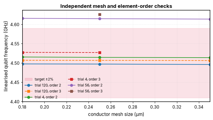
The screening mesh is not a converged frequency limit. A same-geometry refinement check is needed before selection; the figure below shows that the frequency can move enough to change which designs meet the target band. Bulk-silicon \(Q\) changes much less, while interface participation needs its own refinement check near the metal edges.
def site(name: str, default: str) -> str:
    """Return a site setting, letting the environment override the default."""
    return os.environ.get(f"QPDK_{name.upper()}") or default


DEFAULT_SETUP = """
module load python 2>/dev/null || true
export UV_CACHE_DIR="$QPDK_SCRATCH/uv-cache"
export UV_PYTHON_INSTALL_DIR="$QPDK_SCRATCH/uv-python"
export PATH="$PWD/.venv/bin:$HOME/.local/bin:$PATH"
"""

PALACE_SIF = site("palace_sif", site("sif", "/path/to/palace.sif"))

cluster = SlurmCluster(
    partition=site("partition", "batch"),
    scratch=site("scratch", "/scratch/$USER/palace-optimization"),
    setup=site("setup", DEFAULT_SETUP),
    solver_cores=int(site("solver_cores", "8")),
    trial_nodes=int(site("trial_nodes", "4")),
    mem_per_task=site("mem_per_task", "32G"),
    time_limit=site("time_limit", "02:00:00"),
    nodes=int(site("nodes", "4")),
    cores_per_node=int(site("cores_per_node", "8")),
    mem_per_node=site("mem_per_node", "96G"),
    job_name=site("job_name", "qpdk-opt"),
    log_dir=site("log_dir", "slurm-logs"),
    account=site("account", "") or None,
    driver_time_limit=site("driver_time_limit", "24:00:00"),
)
One measured eight-rank screening trial used about 63 GiB. The defaults reserve 96 GiB for each Ray node and 32 GiB per node for a four-node Slurm trial. Check a representative layout before scaling the study.
Running the study#
Optuna proposes layouts and receives each Palace result as soon as its trial finishes. The runner chooses where each independent solve runs:
SlurmRunnersubmits one job per trial.RayRunneruses a reserved Ray allocation.
The runner serialises this notebook’s evaluate_layout function for each
worker. max_in_flight limits concurrent solves.
RUN_ROOT = (
    Path(os.path.expandvars(site("scratch", "build"))) / "palace_optimization_trials"
)


def suggest_layout(trial: optuna.Trial) -> None:
    """Ask Optuna for a candidate geometry, recording it on the trial.

    Suggestions land on the layout grid, so a trial's recorded parameters are
    exactly the geometry that was simulated.
    """
    for name, (low, high) in (
        ("pad_width", PAD_WIDTH_RANGE),
        ("pad_height", PAD_HEIGHT_RANGE),
        ("pad_gap", PAD_GAP_RANGE),
    ):
        trial.suggest_float(name, low, high, step=LAYOUT_GRID_UM)


def objectives(row: dict[str, Any]) -> list[float]:
    """Map one solved trial to the three values the study is ranking.

    Args:
        row: A result row from ``evaluate_layout``.

    Returns:
        Relative frequency error, substrate-limited quality factor, and pad footprint.
    """
    return [
        abs(row["f_linear"] - F_TARGET) / F_TARGET,
        row["quality_factor"],
        row["footprint_mm2"],
    ]


def make_study() -> optuna.Study:
    """Return the multi-objective study this sweep optimises.

    Returns:
        A study ranking frequency error, quality factor and footprint together.
    """
    return optuna.create_study(
        study_name="transmon-layout",
        # Frequency error, then substrate-limited Q, then footprint.
        directions=["minimize", "maximize", "minimize"],
        # NSGA-II keeps a population of non-dominated trials instead of
        # collapsing the objectives into one score.
        sampler=optuna.samplers.NSGAIISampler(seed=0),
    )


# An importable module:function name can still override the notebook evaluator.
EVALUATOR = os.environ.get("QPDK_EVALUATOR") or evaluate_layout


def make_runner() -> SlurmRunner | RayRunner:
    """Return the runner the environment selects.

    Returns:
        A Ray runner when ``QPDK_EXECUTOR=ray``, otherwise a Slurm one.

    Raises:
        ValueError: If a Ray trial needs more cores than one node provides.
    """
    if os.environ.get("QPDK_EXECUTOR") == "ray":
        if cluster.solver_cores > cluster.cores_per_node:
            raise ValueError("Ray trials must fit on one node")
        return RayRunner(
            run_root=RUN_ROOT, ranks=cluster.solver_cores, evaluator=EVALUATOR
        )
    return SlurmRunner(
        cluster=cluster,
        run_root=RUN_ROOT,
        ranks=cluster.solver_cores,
        evaluator=EVALUATOR,
        timeout=6000.0,
    )
Results#
The embedded example replays 150 stored candidate geometries with the exact-gap junction sheet. The live workflow above uses Optuna to generate new candidates. The analysis below reads the saved table without starting a solver.
The recorded bulk screen solves one isolated qubit mode with order-2 elements, a 0.35 µm conductor mesh and a 10 nH junction. Linear-solver and eigenmode tolerances are both \(10^{-5}\). Separate finer-mesh, element-order and domain checks below test the near-target layouts.
2026-10-28 12:26:45.278 | INFO | __main__:<module>:178 - 150 successful trials
Quality factor across the geometry sweep#
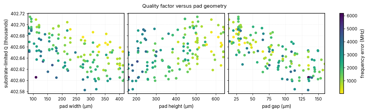
These plots show bulk-silicon \(Q\) against each layout parameter. Colour marks distance from the target frequency. The narrow \(Q\) axis makes small differences visible; the absolute scale appears in the labels.
frames = {
    "pad_width": "pad width (µm)",
    "pad_height": "pad height (µm)",
    "pad_gap": "pad gap (µm)",
}
PARAMETERS = list(frames)
target_ghz = F_TARGET / 1e9
frequency_error_mhz = np.abs(trials["f_linear_ghz"] - target_ghz) * 1e3

fig, axes = plt.subplots(1, 3, figsize=(12, 3.6), sharey=True, constrained_layout=True)
for ax, name in zip(axes, PARAMETERS, strict=True):
    points = ax.scatter(
        trials[name],
        trials["quality_factor"] / 1e3,
        c=frequency_error_mhz,
        cmap="viridis_r",
        s=25,
    )
    ax.set_xlabel(frames[name])
axes[0].set_ylabel("substrate-limited $Q$ (thousands)")
fig.colorbar(points, ax=axes, label="frequency error (MHz)")
fig.suptitle("Quality factor versus pad geometry")
plt.show()
plt.close(fig)
findfont: Failed to find font weight bold, now using 400.
The Pareto frontier#
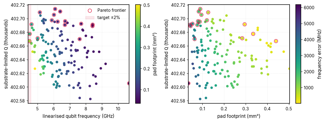
The highlighted designs are not beaten on all three objectives at once: frequency error, bulk-silicon \(Q\), and pad area. Interface loss could change this ordering.
def pareto_mask(values: np.ndarray) -> np.ndarray:
    """Return a mask of rows not dominated when every column is minimised."""
    keep = np.ones(len(values), dtype=bool)
    for i, candidate in enumerate(values):
        dominated = np.all(values <= candidate, axis=1) & np.any(
            values < candidate, axis=1
        )
        if dominated.any():
            keep[i] = False
    return keep


objective_values = np.column_stack([
    frequency_error_mhz,
    -trials["quality_factor"],
    trials["footprint_mm2"],
])
on_front = pareto_mask(objective_values)
front = trials[on_front].sort_values("f_linear_ghz")
logger.info(f"{len(front)} of {len(trials)} trials are on the Pareto frontier")

fig, axes = plt.subplots(1, 2, figsize=(10.8, 4.1))
points = axes[0].scatter(
    trials["f_linear_ghz"],
    trials["quality_factor"] / 1e3,
    c=trials["footprint_mm2"],
    cmap="viridis",
    s=24,
)
axes[0].scatter(
    front["f_linear_ghz"],
    front["quality_factor"] / 1e3,
    facecolors="none",
    edgecolors="crimson",
    s=70,
    label="Pareto frontier",
)
axes[0].axvspan(
    target_ghz * (1 - TOLERANCE_BAND),
    target_ghz * (1 + TOLERANCE_BAND),
    color="crimson",
    alpha=0.1,
    label=f"target ±{TOLERANCE_BAND:.0%}",
)
axes[0].set_xlabel("linearised qubit frequency (GHz)")
axes[0].set_ylabel("substrate-limited $Q$ (thousands)")
axes[0].legend()
fig.colorbar(points, ax=axes[0], label="pad footprint (mm²)")

points = axes[1].scatter(
    trials["footprint_mm2"],
    trials["quality_factor"] / 1e3,
    c=frequency_error_mhz,
    cmap="viridis_r",
    s=24,
)
axes[1].scatter(
    front["footprint_mm2"],
    front["quality_factor"] / 1e3,
    facecolors="none",
    edgecolors="crimson",
    s=70,
)
axes[1].set_xlabel("pad footprint (mm²)")
axes[1].set_ylabel("substrate-limited $Q$ (thousands)")
fig.colorbar(points, ax=axes[1], label="frequency error (MHz)")
fig.tight_layout()
plt.show()
plt.close(fig)
2026-10-28 12:26:45.492 | INFO | __main__:<module>:20 - 17 of 150 trials are on the Pareto frontier
Seeing several dimensions at once#
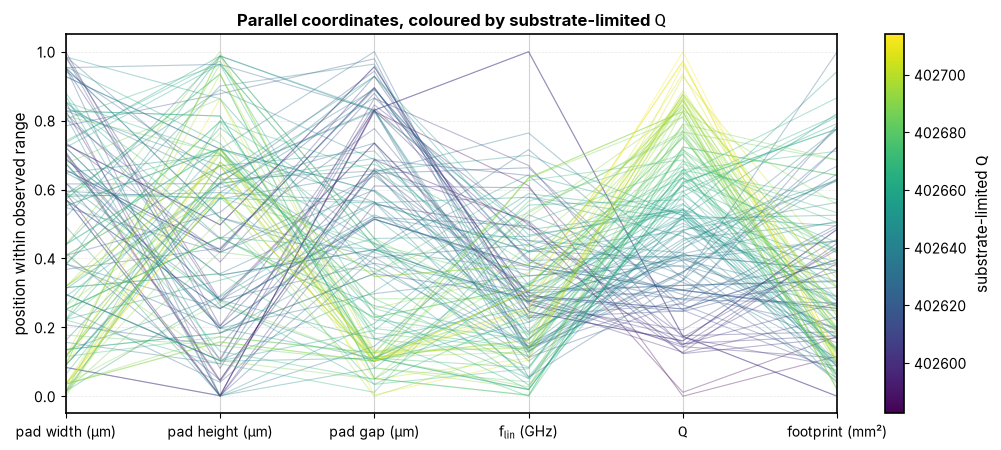
Each line is a trial. Axes are independently scaled to expose trends; the colorbar gives the actual \(Q\) range.
parallel_axes = [*PARAMETERS, "f_linear_ghz", "quality_factor", "footprint_mm2"]
axis_limits = {
    name: (float(trials[name].min()), float(trials[name].max()))
    for name in parallel_axes
}
normaliser = plt.Normalize(
    float(trials["quality_factor"].min()),
    float(trials["quality_factor"].max()),
)
fig, ax = plt.subplots(figsize=(10.5, 4.6))
colors = plt.cm.viridis(normaliser(trials["quality_factor"].to_numpy(dtype=float)))
for row, color in zip(trials.itertuples(), colors, strict=True):
    values = []
    for name in parallel_axes:
        lower, upper = axis_limits[name]
        values.append(
            (getattr(row, name) - lower) / (upper - lower) if upper > lower else 0.5
        )
    ax.plot(
        range(len(parallel_axes)),
        values,
        color=color,
        alpha=0.35,
        lw=0.8,
    )
for index in range(len(parallel_axes)):
    ax.axvline(index, color="0.85", lw=0.8, zorder=0)
ax.set_xticks(range(len(parallel_axes)))
ax.set_xticklabels([
    *[frames[name] for name in PARAMETERS],
    r"$f_\text{lin}$ (GHz)",
    "$Q$",
    "footprint (mm²)",
])
ax.set_ylabel("position within observed range")
ax.set_title("Parallel coordinates, coloured by substrate-limited $Q$")
fig.colorbar(
    plt.cm.ScalarMappable(normaliser, plt.cm.viridis),
    ax=ax,
    label="substrate-limited $Q$",
)
fig.tight_layout()
plt.show()
plt.close(fig)
Frequency and relaxation time#
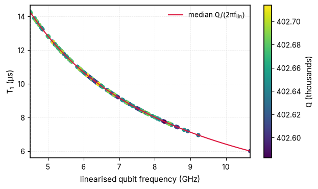
The median-\(Q\) line isolates the \(1/f_\text{lin}\) factor in \(T_1\approx Q/(2\pi f_\text{lin})\). Colour shows each trial’s actual \(Q\).
fig, ax = plt.subplots(figsize=(6.4, 3.8))
points = ax.scatter(
    trials["f_linear_ghz"],
    trials["T1_us"],
    c=trials["quality_factor"] / 1e3,
    cmap="viridis",
    s=25,
)
frequencies = np.linspace(
    trials["f_linear_ghz"].min(), trials["f_linear_ghz"].max(), 200
)
median_q = trials["quality_factor"].median()
ax.plot(
    frequencies,
    median_q / (2 * np.pi * frequencies * 1e3),
    color="crimson",
    label=r"median $Q/(2\pi f_\text{lin})$",
)
ax.axvline(target_ghz, color="0.45", ls="--", lw=1)
ax.set_xlabel("linearised qubit frequency (GHz)")
ax.set_ylabel("$T_1$ (µs)")
ax.legend()
fig.colorbar(points, ax=ax, label="$Q$ (thousands)")
fig.tight_layout()
plt.show()
plt.close(fig)
Screened geometry and finer checks#
The screen keeps candidates near the target frequency, then favours a small footprint among those with similar bulk-silicon \(Q\). Candidate frequencies are checked on finer meshes before a layout is selected.
on_target = trials[
    np.abs(trials["f_linear_ghz"] - target_ghz) < TOLERANCE_BAND * target_ghz
]
if on_target.empty:
    logger.warning(
        f"no trial within {TOLERANCE_BAND:.0%} of {target_ghz} GHz; "
        "falling back to the closest trial"
    )
    on_target = trials.iloc[[int(np.argmin(frequency_error_mhz))]]
best_q = float(on_target["quality_factor"].max())
affordable = on_target[on_target["quality_factor"] >= best_q * (1 - Q_SLACK)]
screen_best = affordable.sort_values("footprint_mm2").iloc[0]
logger.info(
    f"coarse-screen trial {int(screen_best['trial'])}: pads "
    f"{screen_best['pad_width']:.2f} × {screen_best['pad_height']:.2f} µm, "
    f"gap {screen_best['pad_gap']:.2f} µm"
)
logger.info(
    f"f_lin = {screen_best['f_linear_ghz']:.4f} GHz, "
    f"Q = {screen_best['quality_factor']:.1f}, "
    f"T1 = {screen_best['T1_us']:.2f} µs, "
    f"footprint = {screen_best['footprint_mm2']:.3f} mm²"
)
2026-10-28 12:26:45.794 | INFO | __main__:<module>:13 - coarse-screen trial 4: pads 273.14 × 612.80 µm, gap 20.65 µm
2026-10-28 12:26:45.795 | INFO | __main__:<module>:18 - f_lin = 4.5137 GHz, Q = 402677.6, T1 = 14.20 µs, footprint = 0.335 mm²
The 0.35 µm, order-2 screen is a first pass. Separate solves check three near-target layouts at 0.25 and 0.18 µm, then change the element order. Trials 4 and 120 also have lateral-margin and vacuum-height checks. All use the same exact-gap junction sheet and 10 nH inductance. These stored checks refer to the recorded replay. A live study needs independent follow-up solves for its own candidate geometries.
coarse_checks = recorded_trials.loc[
    recorded_trials["trial"].isin(checks["trial"]), ["trial", "f_linear_ghz"]
].assign(mesh_um=0.35, order=2)
coarse_checks["candidate"] = "trial " + coarse_checks["trial"].astype(str)
plotted_checks = pd.concat(
    [coarse_checks, mesh_checks[["candidate", "mesh_um", "order", "f_linear_ghz"]]],
    ignore_index=True,
)
fig, ax = plt.subplots(figsize=(7.2, 4.1))
ax.axhspan(
    target_ghz * (1 - TOLERANCE_BAND),
    target_ghz * (1 + TOLERANCE_BAND),
    color="crimson",
    alpha=0.12,
    label=f"target ±{TOLERANCE_BAND:.0%}",
)
for (candidate, order), group in plotted_checks.groupby(["candidate", "order"]):
    ordered = group.sort_values("mesh_um")
    ax.plot(
        ordered["mesh_um"],
        ordered["f_linear_ghz"],
        "o-" if order == 2 else "s--",
        label=f"{candidate}, order {order}",
    )
ax.set_xlabel("conductor mesh size (µm)")
ax.set_ylabel("linearised qubit frequency (GHz)")
ax.set_title("Independent mesh and element-order checks")
ax.legend(ncol=2, fontsize="small")
fig.tight_layout()
plt.show()
plt.close(fig)
checks.loc[
    checks["trial"].isin([4, 120]),
    ["trial", "mesh_um", "order", "lateral_margin", "vacuum_thickness", "f_linear_ghz"],
].sort_values(["trial", "order", "mesh_um", "lateral_margin", "vacuum_thickness"])
| trial | mesh_um | order | lateral_margin | vacuum_thickness | f_linear_ghz | |
|---|---|---|---|---|---|---|
| 1 | 4 | 0.18 | 2 | 250.0 | 500.0 | 4.515372 |
| 2 | 4 | 0.25 | 2 | 250.0 | 500.0 | 4.514412 |
| 5 | 4 | 0.25 | 2 | 250.0 | 1000.0 | 4.513722 |
| 0 | 4 | 0.25 | 2 | 500.0 | 500.0 | 4.509243 |
| 3 | 4 | 0.18 | 3 | 250.0 | 500.0 | 4.527351 |
| 4 | 4 | 0.25 | 3 | 250.0 | 500.0 | 4.526966 |
| 10 | 120 | 0.18 | 2 | 250.0 | 500.0 | 4.497420 |
| 11 | 120 | 0.25 | 2 | 250.0 | 500.0 | 4.497068 |
| 15 | 120 | 0.25 | 2 | 250.0 | 1000.0 | 4.495668 |
| 9 | 120 | 0.25 | 2 | 500.0 | 500.0 | 4.486455 |
| 12 | 120 | 0.18 | 3 | 250.0 | 500.0 | 4.506910 |
| 13 | 120 | 0.25 | 3 | 250.0 | 500.0 | 4.506667 |
| 14 | 120 | 0.35 | 3 | 250.0 | 500.0 | 4.506247 |
Selection uses the finest order-3 result for each checked layout and requires every saved frequency check to stay inside the target band. That selection supports screening at that band, not a converged mask specification or an absolute lifetime prediction. Small differences in bulk-silicon quality factor should not be read as resolved device-loss improvements.
SELECTION_MESH_UM = 0.18
selected_resolution = mesh_checks[
    (mesh_checks["mesh_um"] == SELECTION_MESH_UM) & (mesh_checks["order"] == 3)
]
band_mhz = TOLERANCE_BAND * target_ghz * 1e3
stays_in_band = checks.groupby("candidate")["target_error_mhz"].apply(
    lambda errors: errors.abs().lt(band_mhz).all()
)
verified_on_target = selected_resolution[
    selected_resolution["candidate"].isin(stays_in_band[stays_in_band].index)
]
assert not verified_on_target.empty, "no candidate stays in the target band"
best_q = float(verified_on_target["dielectric_q"].max())
affordable = verified_on_target[
    verified_on_target["dielectric_q"] >= best_q * (1 - Q_SLACK)
]
best = affordable.sort_values("footprint_mm2").iloc[0]
best_layout = Layout(
    pad_width=float(best["pad_width"]),
    pad_height=float(best["pad_height"]),
    pad_gap=float(best["pad_gap"]),
)
logger.info(
    f"selected recorded candidate at working mesh {best['candidate']}: {best_layout}, "
    f"f_lin = {best['f_linear_ghz']:.4f} GHz at {best['mesh_um']:.3f} µm, "
    f"order {int(best['order'])}, "
    f"substrate Q = {best['dielectric_q']:.1f}, "
    f"footprint = {best['footprint_mm2']:.3f} mm²"
)
best_layout
2026-10-28 12:26:45.966 | INFO | __main__:<module>:23 - selected recorded candidate at working mesh trial 4: Layout(pad_width=273.14, pad_height=612.8, pad_gap=20.65), f_lin = 4.5274 GHz at 0.180 µm, order 3, substrate Q = 402682.5, footprint = 0.335 mm²
Layout(pad_width=273.14, pad_height=612.8, pad_gap=20.65)
Interface participation#
Separate Palace solves add 3 nm substrate-air (SA), metal-substrate (MS), and metal-air (MA) dielectric sheets with relative permittivity 10. These first-order solves reuse the refined layout meshes but have lower basis order than the main sweep to stay within moderate memory. Their participations are screening diagnostics, not inputs to the bulk-loss Pareto frontier.
fig, axes = plt.subplots(1, 3, figsize=(12, 3.6), sharey=True, constrained_layout=True)
for ax, name in zip(axes, PARAMETERS, strict=True):
    for kind, label, color, marker in (
        ("sa", "substrate-air", "#009E73", "o"),
        ("ms", "metal-substrate", "#0072B2", "s"),
        ("ma", "metal-air", "#CC79A7", "^"),
    ):
        ax.scatter(
            interfaces[name],
            interfaces[f"participation_{kind}"],
            label=label,
            color=color,
            marker=marker,
            s=34,
        )
    ax.set_xlabel(frames[name])
axes[0].set_yscale("log")
axes[0].set_ylabel("3 nm interface participation")
axes[-1].legend(loc="upper right", fontsize="small")
fig.suptitle("Interface electric-energy participation")
plt.show()
plt.close(fig)
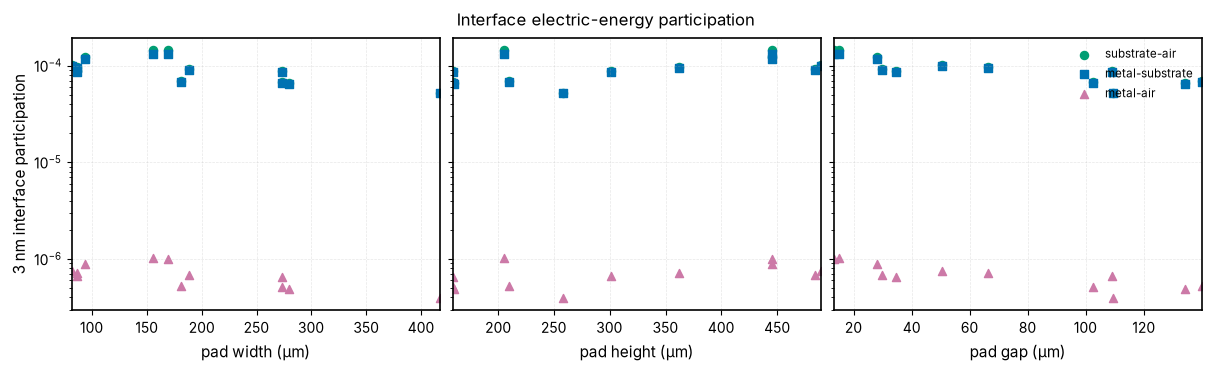
These values depend on near-metal mesh resolution and sheet assumptions. A loss tangent for each interface is needed to turn them into an interface quality factor.
Running the study on a Slurm cluster#
SlurmCluster writes one trial job per geometry and a driver that keeps a
bounded number of jobs in flight. Site settings come from the QPDK_*
environment variables in site() above. A Ray script is available for
allocations that reserve their nodes together.
driver = (
    f"export QPDK_RUN_OPTIMIZATION=1 "
    f"QPDK_N_TRIALS={N_TRIALS} QPDK_MAX_IN_FLIGHT={MAX_IN_FLIGHT} "
    f"QPDK_PALACE_SIF={shlex.quote(PALACE_SIF)} QPDK_TRIALS_CSV=trials.csv\n"
    "uv run --frozen python notebooks/src/palace_batched_qubit_optimization.py"
)

driver_path = cluster.write_driver_script("build/submit_driver.sbatch", driver)
logger.info(f"wrote {driver_path}")
2026-10-28 12:26:46.117 | INFO | __main__:<module>:9 - wrote build/submit_driver.sbatch
Ray uses one allocation for its driver and workers. Use it to group short trials into hour-plus batches. Its walltime covers the full study.
if cluster.solver_cores <= cluster.cores_per_node:
    ray_driver = (
        f"export QPDK_RUN_OPTIMIZATION=1 QPDK_EXECUTOR=ray "
        f"QPDK_N_TRIALS={N_TRIALS} QPDK_MAX_IN_FLIGHT={MAX_IN_FLIGHT} "
        f"QPDK_PALACE_SIF={shlex.quote(PALACE_SIF)} QPDK_TRIALS_CSV=trials.csv\n"
        "uv run --frozen python notebooks/src/palace_batched_qubit_optimization.py"
    )
    ray_cluster = replace(cluster, time_limit=cluster.driver_time_limit)
    ray_path = ray_cluster.write_sbatch_script("build/submit_ray.sbatch", ray_driver)
    logger.info(f"wrote {ray_path}")
else:
    logger.info("Ray needs each trial to fit on one node")
2026-10-28 12:26:46.121 | INFO | __main__:<module>:10 - wrote build/submit_ray.sbatch
Submit the driver and follow its log:
sbatch build/submit_driver.sbatch
tail -f slurm-logs/*-driver-*.out
Check a known geometry and size the allocation from its measured memory use before launching the full sweep.
Summary#
The Pareto frontier keeps frequency error, bulk-loss \(Q\), and footprint separate. The parallel-coordinates plot exposes their geometry dependence.
\(T_1=Q/(2\pi f_\text{lin})\) falls with frequency even when \(Q\) barely changes. Thin-interface participation is examined separately above and has no assumed loss tangent in the Pareto objective.
These are simulated screening results, not absolute device lifetimes.
References#
Niko Savola. Design and modelling of long-coherence qubits using energy participation ratios. Master's thesis, Aalto University, February 2023. URN:NBN:fi:aalto-202305213270.