Palace Eigenmode Simulation of a Transmon with a Readout Resonator#

This notebook demonstrates a full-wave eigenmode simulation of a double-pad transmon qubit capacitively coupled to a quarter-wave CPW readout resonator and read through a probeline, using Palace, an open-source parallel 3-D finite-element electromagnetic solver, driven through gsim. It is the open-source counterpart of the HFSS Eigenmode Simulation of a CPW Resonator notebook: same physics, no commercial solver license.

The workflow goes from layout to nearby qubit and readout eigenmodes, with an analytical CPW estimate as a cross-check:

        flowchart TB
    A["Layout<br>(qpdk cells)"]
    B["FEM regions<br>(subtractive mask to explicit conductor)"]
    C["Analytical estimate<br>(CPW cross-section)"]
    D["Eigenmode setup and mesh<br>(gsim, Gmsh)"]
    E["Palace solve<br>(cluster)"]
    F["Eigenmodes vs. estimate"]
    G["Check participation, fields, and mesh sensitivity"]
    A --> B --> D --> E --> F --> G
    C --> F

Eigenmode analysis is the workhorse behind quantitative qubit design: the linearized eigenfrequencies and eigenfields of the Josephson circuit, with the junction treated as a lumped inductor, determine the system Hamiltonian once completed with the junction’s energy participation [MLM+21, NPV+12]. Here we stop at the classical part: eigenfrequencies and quality factors.

Required extras

This notebook needs the models extra:

uv add "qpdk[models]"
# or, from a checkout of this repository:
uv sync --extra models --group palace
# or with pip:
pip install "qpdk[models]"

The layout and setup cells also need gsim. The palace dependency group installs the pinned version used here. The standalone script and Colab setup install that same revision. Palace itself is an external executable. Its mesh and solve calls are fenced examples, and the saved results let the analysis run without launching a solver.

See the extras reference for what each extra installs.

The results shown below were produced with Palace on an HPC cluster; the solver data is embedded in hidden cells so the rendered docs show the analysis, not the raw tables.

Simulation layout#

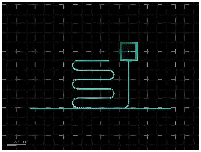
The device is the transmon_with_resonator_and_probeline() cell: a double-pad transmon, a meandered quarter-wave CPW resonator coupled to one pad, and a probeline feed coupled along the readout line. It exposes exactly the ports a 3-D solve needs:

junction: the position of the Josephson junction between the two qubit pads, which becomes the lumped inductive port.
coupling_o1 / coupling_o2: the two ends of the probeline feed, which become 50 Ω CPW lumped ports.

The cell’s resonator_length includes the meander, probeline coupling section, and qubit-side route. The conductor is shorted at the far end of the meander and open at the plate facing the qubit. The route is already in the length used for the quarter-wave estimate below.

Two details need care when the cell is used standalone:

The meander’s far end must reach ground. The qubit-side plate stays open, outside the qubit etch, and separated from the pads by a capacitive gap.
Bare probeline port ends touch ground at their end faces, so the wrapper extends the gap etch past both feed ends.

A SIM_AREA rectangle bounds the silicon and vacuum volumes. The default ground margin is 500 µm, and each probeline end extends another 1000 µm beyond the coupling section. The 150 × 300 µm pads retain a 15 µm junction gap. Junction inductance sets their frequency after the pad size changes.

# The cell uses this total to size the meander after laying out the separate
# coupling section and qubit-side arm.
RESONATOR_LENGTH = 7020.0  # µm
RESONATOR_MEANDERS = 5
RESONATOR_MEANDER_START = (-1100.0, -1200.0)  # µm
QUBIT_PAD_SIZE = (150.0, 300.0)  # µm
QUBIT_PAD_GAP = 15.0  # µm
QUBIT_BBOX_EXTENSION = 40.0  # µm
GROUND_MARGIN = 500.0  # µm
PROBELINE_EXTENSION = 1000.0  # µm per end
JUNCTION_INDUCTANCE = 2.515e-08  # H
JUNCTION_PORT_WIDTH = 2.0  # µm
JUNCTION_PORT_LENGTH = QUBIT_PAD_GAP
NEAR_MESH = 0.55  # µm
ELEMENT_ORDER = 3
COUPLER_WIDTH = 10.0  # µm
COUPLER_LENGTH = 120.0  # µm
COUPLER_OFFSET = (-QUBIT_BBOX_EXTENSION - 6.0, 0.0)  # µm
COUPLER_ETCH_MARGIN = 2.0  # µm


@gf.cell
def qubit_resonator_sim_component(
    resonator_length: float = RESONATOR_LENGTH,
    meanders: int = RESONATOR_MEANDERS,
    pad_size: tuple[float, float] = QUBIT_PAD_SIZE,
    ground_margin: float = GROUND_MARGIN,
    probeline_extension: float = PROBELINE_EXTENSION,
) -> gf.Component:
    """Transmon, resonator and probeline wrapped with a simulation area.

    Args:
        resonator_length: Layout length budget used to size the meander in µm.
        meanders: Number of meander sections.
        pad_size: Dimensions of each qubit pad in µm.
        ground_margin: Ground clearance around the extended layout in µm.
        probeline_extension: Extra CPW length at each feed end in µm.

    Returns:
        Component with the simulation layout and ports
        ``junction``, ``coupling_o1``, ``coupling_o2``.
    """
    c = gf.Component()

    ref = c << transmon_with_resonator_and_probeline(
        qubit=partial(
            double_pad_transmon_with_bbox,
            pad_size=pad_size,
            pad_gap=QUBIT_PAD_GAP,
            bbox_extension=QUBIT_BBOX_EXTENSION,
        ),
        coupler=partial(
            plate_capacitor_single,
            width=COUPLER_WIDTH,
            length=COUPLER_LENGTH,
            etch_bbox_margin=COUPLER_ETCH_MARGIN,
        ),
        coupler_offset=COUPLER_OFFSET,
        resonator_length=resonator_length,
        resonator_meanders=meanders,
        resonator_meander_start=RESONATOR_MEANDER_START,
        # The open end is the plate at the qubit; this bare meander end meets ground.
        resonator_open_end=False,
        qubit_rotation=90,
    )
    junction = ref.ports["junction"]
    c.add_port(
        "junction",
        center=junction.center,
        width=JUNCTION_PORT_WIDTH,
        orientation=junction.orientation,
        layer=junction.layer,
        port_type=junction.port_type,
    )
    c.add_ports(ref.ports.filter(regex=r"^(?!junction$|coupling_o[12]$)"))
    routed = ref.cell.info["length"]
    assert abs(routed - resonator_length) < 1.0, (
        f"cell routed {routed} µm, expected {resonator_length} µm"
    )
    c.info["routed_length"] = routed
    meander_ref = next(
        inst
        for inst in ref.cell.insts
        if inst.cell.info.get("resonator_type") == "quarter_wave"
    )
    c.info["meander_length"] = meander_ref.cell.info["length"]
    qubit_ref, coupler_ref = list(ref.cell.insts)[:2]
    assert (
        coupler_ref.dbbox().top - COUPLER_ETCH_MARGIN
        < qubit_ref.dbbox().bottom
        < coupler_ref.dbbox().top
    ), "open-end metal must stay outside the qubit etch while the etch windows meet"
    assert (
        qubit_ref.ports["left_pad"].y - (coupler_ref.dbbox().top - COUPLER_ETCH_MARGIN)
        >= 20
    ), "the open end is too close to the qubit pad"
    assert meander_ref.dbbox().right < coupler_ref.ports["o1"].x - 30, (
        "the meander crosses the qubit-side route"
    )
    for name in ("coupling_o1", "coupling_o2"):
        port = ref.ports[name]
        if probeline_extension:
            feed = c << straight(length=probeline_extension, cross_section="cpw")
            feed.connect("o1", port)
            port = feed.ports["o2"]
        c.add_port(name, port=port)
        # Leave an etched clearance behind the matched load.
        ext = c << straight(length=10.0, cross_section="etch")
        ext.connect("o1", port, allow_layer_mismatch=True)

    c.kdb_cell.shapes(gf.get_layer(LAYER.SIM_AREA)).insert(
        c.bbox().enlarged(ground_margin, ground_margin)
    )
    return c


component = qubit_resonator_sim_component()
component.plot()
logger.info(f"Ports: {[p.name for p in component.ports]}")
bounds = component.dbbox()
logger.info(f"Simulation footprint: {bounds.width():.0f} × {bounds.height():.0f} µm")

2026-10-27 15:15:13.296 | INFO     | __main__:<module>:119 - Ports: ['junction', 'o1', 'coupling_o1', 'coupling_o2']

2026-10-27 15:15:13.297 | INFO     | __main__:<module>:121 - Simulation footprint: 4020 × 2434 µm

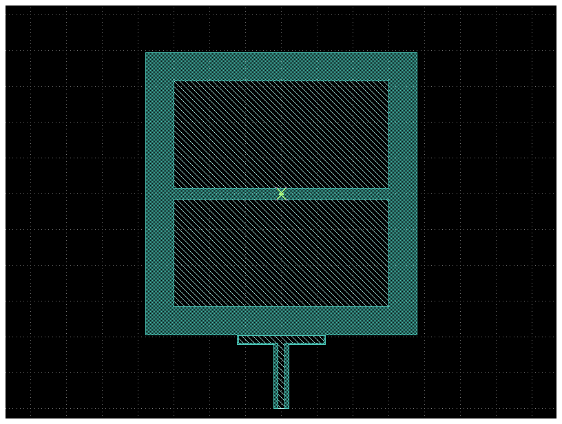
../_images/2e217f3a11eada39ebe4b617a75a44176ae6a364555501eb85bf67b417e4c659.png

The close view shows the 10 µm wide readout plate below the qubit’s etched box. Its own etch joins that box, but the metal stays outside it and at least 20 µm from the qubit pad. The trace continues down to the meander, whose opposite end terminates on the ground plane.

qubit_close_view = gf.Component()
qubit_close_view << component
qubit_close_view.trim(left=-230, bottom=-300, right=230, top=250, flatten=True)
qubit_close_view.plot(show_labels=False, show_ruler=False)

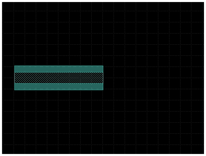
../_images/cf8d2410cf40f7585bcfaaee1621821dba7fcf9f6fc69748b5f6f2a03494796c.png

At the opposite end, the meander etch stops at the trace end. The conductor therefore joins the surrounding ground plane there, providing the short of the quarter-wave resonator.

device_ref = next(iter(component.insts))
meander_ref = next(
    inst
    for inst in device_ref.cell.insts
    if inst.cell.info.get("resonator_type") == "quarter_wave"
)
short_x, short_y = meander_ref.ports["o2"].center
short_close_view = gf.Component()
short_close_view << component
short_close_view.trim(
    left=short_x - 80,
    bottom=short_y - 65,
    right=short_x + 80,
    top=short_y + 65,
    flatten=True,
)
short_close_view.plot(show_labels=False, show_ruler=False)

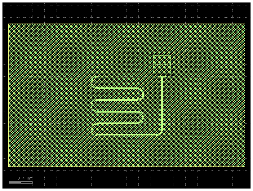
../_images/7e0982bff82be3e0901486c084a59d1923d1a388d7fc1b3d061b291a4769847e.png

From etch layers to simulation regions#

qpdk draws metal subtractively, but a volumetric solver needs explicit conductor and dielectric bodies; to_fem_regions() converts between the two with SIM_AREA - (M1_ETCH - M1_DRAW). From etch layers to simulation regions works through the conversion with a picture, including what it does to an additive shape sitting inside an etched gap.

etched = to_fem_regions(component)
metal = kdb.Region(
    etched.kdb_cell.begin_shapes_rec(
        etched.kdb_cell.layout().layer(*FEM_LAYERS["SUPERCONDUCTOR"])
    )
).merged()
assert len(metal) == 4, "expected the grounded readout, feed, and two qubit pads"
islands = list(metal)


def _metal_island(x: float, y: float) -> int:
    point = kdb.Point(round(x / etched.kcl.dbu), round(y / etched.kcl.dbu))
    matches = [index for index, polygon in enumerate(islands) if polygon.inside(point)]
    assert len(matches) == 1, f"expected one conductor at ({x}, {y}), got {matches}"
    return matches[0]


ground = _metal_island(component.dbbox().left + 5, component.dbbox().top - 5)
readout = _metal_island(*component.ports["o1"].center)
feed1 = component.ports["coupling_o1"].center
feed2 = component.ports["coupling_o2"].center
feed = _metal_island((feed1[0] + feed2[0]) / 2, (feed1[1] + feed2[1]) / 2)
pad_centres = (QUBIT_PAD_SIZE[0] + QUBIT_PAD_GAP) / 2
pad1 = _metal_island(0, -pad_centres)
pad2 = _metal_island(0, pad_centres)
assert readout == ground, "the far end of the readout must meet ground"
assert len({readout, feed, pad1, pad2}) == 4, (
    "the readout must stay separate from the feed and both qubit pads"
)

# The cell's ``junction`` port is a *placement* marker: it points along the
# junction wire, which the transmon cells build perpendicular to the pad-to-pad
# axis (``left_pad_inner`` and ``right_pad_inner`` face each other across the
# gap, while the junction port sits at the gap centre at 90° to them). A lumped
# port has to bridge pad to pad, so rotate by that 90°. Deriving it this way
# rather than hard-coding an angle keeps it correct for any ``qubit_rotation``.
etched.ports["junction"].orientation = (
    etched.ports["junction"].orientation + 90.0
) % 360.0

junction_sheet = kdb.Region(
    kdb.DBox(
        -JUNCTION_PORT_WIDTH / 2,
        -JUNCTION_PORT_LENGTH / 2,
        JUNCTION_PORT_WIDTH / 2,
        JUNCTION_PORT_LENGTH / 2,
    ).to_itype(etched.kcl.dbu)
)
assert (junction_sheet & metal).is_empty(), "junction sheet overlaps pad metal"
assert len(metal.interacting(junction_sheet.sized(1))) == 2, (
    "junction sheet must touch both pad edges"
)

etched.plot()

../_images/993f5152ddd8a7d4a1848ee2d7021fe4165e6d63bb7b7ca5da56f1aafc05198a.png

Analytical resonator estimate#

The CPW cross-section model gives a first estimate of the readout frequency before any mesh is built. A quarter-wave resonator of length \(L\) resonates at \(f_\text{r} = v_\text{p} / 4L\) with phase velocity \(v_\text{p} = c_0 / \sqrt{\varepsilon_{\text{eff}}}\), where \(\varepsilon_{\text{eff}}\) comes from the conformal-mapping CPW model in cpw_parameters() [MP12, Sim01].

RESONATOR_CROSS_SECTION = "cpw"

width, gap = get_cpw_dimensions(RESONATOR_CROSS_SECTION)
epsilon_eff, z0 = cpw_parameters(width, gap)
logger.info(f"CPW width {width} µm, gap {gap} µm")
logger.info(
    f"ε_eff = {float(np.real(epsilon_eff)):.3f}, Z0 = {float(np.real(z0)):.1f} Ω"
)

routed_length = component.info["routed_length"]
pdk_analytical_freq = resonator_frequency(
    length=routed_length,
    cross_section=RESONATOR_CROSS_SECTION,
    is_quarter_wave=True,
)
epsilon_eff_sheet = cpw_epsilon_eff(
    width * 1e-6,
    gap * 1e-6,
    500e-6,
    material_properties["Si"]["relative_permittivity"],
)
analytical_freq = c_0 / float(epsilon_eff_sheet) ** 0.5 / (4 * routed_length * 1e-6)
logger.info(
    f"Routed length {routed_length:.1f} µm, PEC-sheet quarter-wave estimate "
    f"{analytical_freq / 1e9:.4f} GHz"
)
logger.info(f"Finite-thickness PDK estimate: {pdk_analytical_freq / 1e9:.4f} GHz")

2026-10-27 15:15:14.371 | INFO     | __main__:<module>:5 - CPW width 10.0 µm, gap 6.0 µm

2026-10-27 15:15:14.393 | INFO     | __main__:<module>:6 - ε_eff = 6.065, Z0 = 49.3 Ω

2026-10-27 15:15:14.441 | INFO     | __main__:<module>:23 - Routed length 7020.0 µm, PEC-sheet quarter-wave estimate 4.2793 GHz

2026-10-27 15:15:14.441 | INFO     | __main__:<module>:27 - Finite-thickness PDK estimate: 4.3351 GHz

Both estimates use the actual routed CPW length. The PDK model includes the 200 nm metal thickness, while Palace uses a zero-thickness PEC sheet. Matching that assumption lowers the estimate from 4.3351 to 4.2793 GHz. Neither formula includes the open-end plate, feed and qubit loading, or the bends. The plate is a capacitive termination, not another length of uniform CPW.

Junction-sheet geometry#

The electrical sheet ends at the pad edges. Extending it over the pads removes PEC boundary coverage from the overlap patches in the generated mesh, even though the positive-metal polygons still look intact. Checking those polygons alone does not establish correct electrical contact.

With the enlarged layout, a 0.70 µm mesh, order 2 and 10 nH held fixed:

sheet length (µm)	sheet width (µm)	junction-sensitive pole (GHz)	readout (GHz)	reported \(\lvert p_\text{J}\rvert\)
25	33.446	2.235890	4.189576	0.1215
15	33.446	6.323322	4.189379	0.9961
15	2	6.324632	4.189368	0.9950

The overlapping sheet’s weakly participating branch is not used for tuning. The setup uses an exact-gap sheet and a narrow 2 µm electrical width, independent of the junction’s wider layout-placement marker. The readout moves by only 0.20 MHz in this off-resonant control, so this port issue is separate from the much larger CPW-estimate offset.

Eigenmode setup with gsim#

gsim turns the converted layout into a 3-D model: a LayerStack assigns each GDS layer a material and a z-extent, and EigenmodeSim configures the ports and the eigenmode search. The setup is shown as code without meshing during notebook execution; gsim and Palace are installed separately. The configuration matches the saved solve below.

import json

from gsim.palace import EigenmodeSim

from qpdk.simulation import single_chip_stack

# 500 µm of microwave silicon and 500 µm of air above it; the substrate
# uses the qpdk material properties (eps_r = 11.45, tan d = 2.7e-6), so the
# FEM models the same chip as the analytical CPW models of the previous
# section.
stack = single_chip_stack(substrate_thickness=500.0, vacuum_thickness=500.0)

sim = EigenmodeSim()
sim.set_geometry(etched)
sim.set_stack(stack)
sim.set_solver(order=ELEMENT_ORDER, solver_type="MUMPS")

# Retune the linear junction inductance for the enlarged pads.
# resistance=0 overrides the R = 50 Ω that gsim's default
# port impedance would emit: the linearized junction is purely reactive, so
# it shifts the qubit-like mode but adds no dissipation. The narrow sheet
# joins the pad edges across the 15 µm gap. Its electrical width is separate
# from the wider junction placement marker in the layout cell.
sim.add_port(
    "junction",
    layer="SUPERCONDUCTOR",
    length=JUNCTION_PORT_LENGTH,
    inductance=JUNCTION_INDUCTANCE,
    resistance=0.0,
)

# Probeline feeds as 50 Ω CPW lumped ports, one per end.
sim.add_cpw_port("coupling_o1", layer="SUPERCONDUCTOR", s_width=10.0, gap_width=6.0, length=5.0)
sim.add_cpw_port("coupling_o2", layer="SUPERCONDUCTOR", s_width=10.0, gap_width=6.0, length=5.0)

# Search below the pair so mesh shifts do not exclude the qubit mode.
sim.set_eigenmode(target=3500000000.0, num_modes=2, save=2)

sim.set_output_dir("./sim_palace_qubit_resonator")
sim.mesh(preset="default", refined_mesh_size=NEAR_MESH, auto_size=False)
sim.write_config()
config_path = Path("sim_palace_qubit_resonator/config.json")
config = json.loads(config_path.read_text())
config["Solver"]["Linear"].update({
    "Tol": 1e-5,
    "MaxIts": 20,
    "MGMaxLevels": ELEMENT_ORDER,
    "PCMatReal": False,
    "PCMatShifted": False,
    "ComplexCoarseSolve": True,
    "ColumnOrdering": "ParMETIS",
})
config["Solver"]["Eigenmode"]["Tol"] = 1e-5
config_path.write_text(json.dumps(config, indent=2))

Four details of this setup:

The substrate carries the qpdk microwave-silicon loss tangent (\(\tan\delta = 2.7 \times 10^{-6}\) [CFL+22]), which contributes to the mode loss budget below.
The junction port makes the qubit participate in the linear spectrum: the capacitance between the pads comes from the field solution, the inductive part from the port. Its isolated linear LC estimate is \(f_\text{q} \approx 1 / (2\pi\sqrt{L_\text{J} C_\Sigma})\) [KYG+07, KKY+19].
Unspecified exterior boundaries use Palace’s natural PMC condition, which sets the tangential magnetic field to zero. This finite-domain calculation does not model radiation loss into open space.
sim.mesh() and sim.write_config() leave a self-contained mesh and Palace configuration that can be solved with MPI.

Solving with Palace#

The saved result used 64 MPI ranks. The mesh and configuration can be solved with any compatible Palace build:

cd <simulation directory>  # config.json + palace.msh
mpirun -np 64 palace-x86_64.bin config.json

refined_mesh_size is the knob that matters for field quality: it sets the element size near the conductors, where the field varies fastest. The comparison below checks sensitivity to mesh size and element order before interpreting the mode spacing.

Palace writes one row per mode to output/palace/eig.csv: mode index, the real and imaginary parts of the eigenfrequency in GHz, and the quality factor. Two companion tables make mode identification quantitative: output/palace/port-EPR.csv for the energy-participation ratio of each lumped port in each mode and output/palace/port-Q.csv for the external quality factor per port. The solved rows are embedded below so the analysis runs without the output files.

Results: eigenmodes versus the analytical estimate#

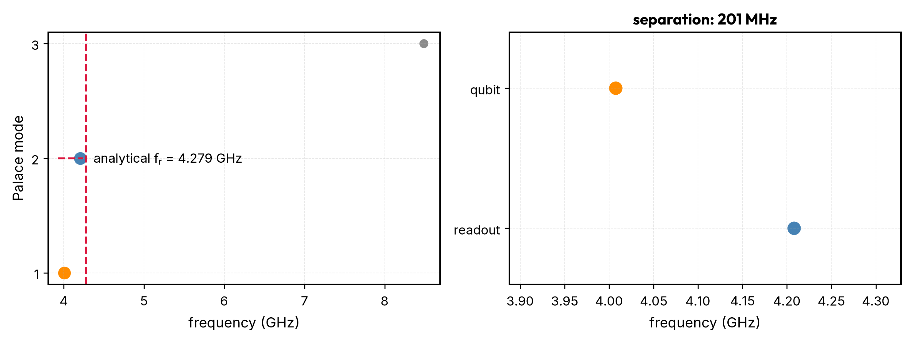
The meander, feed coupling section, and qubit-side route form a single quarter-wave line with a 7020 µm routed length. Among the returned modes, identify the qubit-like mode set by the junction inductance and pad capacitance, and the dressed readout resonance near the analytical estimate. Frequencies and separations below refer to the linearized eigenproblem.

2026-10-27 15:15:14.447 | INFO     | __main__:<module>:13 -   m  Re{f} (GHz)      Q_raw         p_J       Q_ext

2026-10-27 15:15:14.447 | INFO     | __main__:<module>:17 -   1       4.0074   1.51e+05   -9.87e-01    2.56e+05

2026-10-27 15:15:14.448 | INFO     | __main__:<module>:17 -   2       4.2081   2.54e+03   -1.08e-02    2.57e+03

2026-10-27 15:15:14.448 | INFO     | __main__:<module>:17 -   3       8.4870   6.05e+02    5.55e-09    5.76e+02

Three features identify the modes, and they must agree:

Frequency: the qubit and readout form a nearby pair; the analytical quarter-wave estimate is only a starting point for the readout.
Junction participation: port-EPR.csv reports the fraction \(p_{m,\text{J}}\) of each mode’s energy stored in the junction port [MLM+21]. The qubit-like mode carries by far the largest participation; a resonator-like mode keeps most of its inductive energy in the CPW trace and participates much less.
Port dissipation: port-Q.csv gives the external quality factor of each mode through the 50 Ω probeline ports. The readout resonance couples to the feedline and gets a finite \(Q_{\text{ext}}\) (with both feed ports adding in parallel, \(1/Q = 1/Q_{\text{diel}} + \sum 1/Q_{\text{ext}}\)). The nearby qubit-like mode couples more weakly to the feedline, though its external loss need not be negligible at this small detuning. Silicon loss alone would give \(Q_{\text{diel}} \approx 1 / (p_{\text{diel}} \tan\delta)\) with \(\tan\delta = 2.7 \times 10^{-6}\).

No single feature suffices: a heavily feed-coupled spurious mode can have the lowest Q of the spectrum without being the readout resonance. Participation-based identification is the standard in quantitative qubit design: the same EPRs that label the modes also turn the eigenmode data into a quantum Hamiltonian with anharmonicities and couplings [MLM+21, NPV+12]. The stored port values serve as mode-identification diagnostics here. Energy normalization and loss convergence remain separate checks for a Hamiltonian or lifetime extraction.

analytical_ghz = analytical_freq / 1e9
# A higher harmonic can carry more junction energy than the fundamental.
JUNCTION_PARTICIPATION_FLOOR = 0.5
_candidates = np.flatnonzero(np.abs(junction_epr) >= JUNCTION_PARTICIPATION_FLOOR)
assert _candidates.size, "no strongly junction-participating qubit mode"
i_qubit = int(_candidates[np.argmin(eig_f_re[_candidates])])
_readout_candidates = np.flatnonzero(np.abs(junction_epr) < 0.05)
assert _readout_candidates.size, "no mode with low junction participation"
i_res = int(
    _readout_candidates[
        np.argmin(np.abs(eig_f_re[_readout_candidates] - analytical_ghz))
    ]
)
resonator_fem_ghz = eig_f_re[i_res]
resonator_q = eig_q[i_res]
assert abs(junction_epr[i_res]) < 0.05, (
    "identified readout mode stores too much junction energy"
)
logger.info(f"Analytical estimate:          {analytical_ghz:.4f} GHz")
logger.info(
    f"Palace readout resonance:     {resonator_fem_ghz:.4f} GHz "
    f"(mode {eig_m[i_res]}, p_J = {junction_epr[i_res]:.2e})"
)
logger.info(
    f"Relative offset:              "
    f"{(resonator_fem_ghz - analytical_ghz) / analytical_ghz:+.2%}"
)
effective_length_um = routed_length * analytical_ghz / resonator_fem_ghz
logger.info(
    f"Equivalent electrical length: {effective_length_um:.1f} µm "
    f"({effective_length_um - routed_length:+.1f} µm over the routed line)"
)
logger.info(
    f"Readout raw quality factor:   {resonator_q:.3e} "
    f"(Q_ext = {q_ext_feed[i_res]:.3e} through both feed ports)"
)
logger.info(
    f"Qubit-like mode:              {eig_f_re[i_qubit]:.4f} GHz "
    f"(mode {eig_m[i_qubit]}, p_J = {junction_epr[i_qubit]:.2e})"
)
logger.info(
    f"Qubit-readout separation:    "
    f"{abs(resonator_fem_ghz - eig_f_re[i_qubit]) * 1e3:.1f} MHz"
)

fig, axes = plt.subplots(1, 2, figsize=(10, 3.8))
axes[0].scatter(eig_f_re, eig_m, color="0.55", s=36)
axes[0].scatter(eig_f_re[i_qubit], eig_m[i_qubit], color="darkorange", s=80)
axes[0].scatter(eig_f_re[i_res], eig_m[i_res], color="steelblue", s=80)
axes[0].axvline(
    analytical_ghz,
    color="crimson",
    linestyle="--",
    label=rf"analytical $f_\text{{r}}$ = {analytical_ghz:.3f} GHz",
)
axes[0].set_xlabel("frequency (GHz)")
axes[0].set_ylabel("Palace mode")
axes[0].set_yticks(eig_m)
axes[0].set_xlim(min(analytical_ghz, eig_f_re.min()) - 0.2, eig_f_re.max() + 0.2)
axes[0].legend(loc="center left")
axes[1].scatter(
    [eig_f_re[i_qubit], resonator_fem_ghz],
    [1, 0],
    color=["darkorange", "steelblue"],
    s=90,
)
axes[1].set_yticks([0, 1], ["readout", "qubit"])
axes[1].set_xlim(
    min(eig_f_re[i_qubit], resonator_fem_ghz) - 0.12,
    max(eig_f_re[i_qubit], resonator_fem_ghz) + 0.12,
)
axes[1].set_ylim(-0.4, 1.4)
axes[1].set_xlabel("frequency (GHz)")
axes[1].set_title(
    f"separation: {abs(resonator_fem_ghz - eig_f_re[i_qubit]) * 1e3:.0f} MHz"
)
fig.tight_layout()
plt.show()
plt.close(fig)

2026-10-27 15:15:14.456 | INFO     | __main__:<module>:19 - Analytical estimate:          4.2793 GHz

2026-10-27 15:15:14.457 | INFO     | __main__:<module>:20 - Palace readout resonance:     4.2081 GHz (mode 2, p_J = -1.08e-02)

2026-10-27 15:15:14.457 | INFO     | __main__:<module>:24 - Relative offset:              -1.66%

2026-10-27 15:15:14.457 | INFO     | __main__:<module>:29 - Equivalent electrical length: 7138.8 µm (+118.8 µm over the routed line)

2026-10-27 15:15:14.458 | INFO     | __main__:<module>:33 - Readout raw quality factor:   2.541e+03 (Q_ext = 2.571e+03 through both feed ports)

2026-10-27 15:15:14.458 | INFO     | __main__:<module>:37 - Qubit-like mode:              4.0074 GHz (mode 1, p_J = -9.87e-01)

2026-10-27 15:15:14.458 | INFO     | __main__:<module>:41 - Qubit-readout separation:    200.6 MHz

../_images/e11f487f736f5403ac2e7929dec7663be9f09728ed5211bf56270da132199f34.png

Mesh and element-order sensitivity#

Hold the enlarged geometry and 25.15 nH junction fixed while changing the near-conductor mesh size and polynomial order. The rows below are separate solves of the exact-gap sheet model.

mesh size (µm)	order	qubit (GHz)	readout (GHz)	separation (MHz)
0.70	2	3.990952	4.191883	200.931
0.55	2	3.993232	4.195651	202.420
0.70	3	4.006395	4.206422	200.027
0.55	3	4.007439	4.208078	200.639

The mode spacing stays within 2 MHz of 201 MHz, close to the original 205 MHz target. At 0.55 µm, increasing the order moves the two frequencies by 14.2 and 12.4 MHz. At order 3, refining from 0.70 to 0.55 µm changes them by 1.0 and 1.7 MHz. Absolute frequencies still need tighter convergence before setting a design tolerance. Quality factors remain loss diagnostics at this eigensolver tolerance.

Ground and domain sensitivity#

The enlarged layout has separate domain checks at order 2 and 0.55 µm, with the exact-gap junction sheet and 25.15 nH held fixed:

ground/domain margin (µm)	vacuum height (µm)	qubit (GHz)	readout (GHz)	separation (MHz)
500	500	3.993232	4.195651	202.420
1000	500	3.993259	4.195621	202.362
500	1000	3.993157	4.195817	202.660

Doubling the ground margin changes the readout by 0.03 MHz, and doubling the vacuum height changes it by 0.17 MHz. Both changes move each mode by less than 0.2 MHz, below the observed mesh and element-order shifts. These checks support the 500 µm ground margin and 500 µm vacuum height.

To test the original ground-plane hypothesis, hold the 55 × 110 µm pads, original overlapping junction sheet at 10 nH, 7020 µm CPW route and unextended feed fixed. Only the readout branch is used for these diagnostics. Separate order-2, 0.55 µm runs change the lateral ground and simulation-area margin together. Silicon and vacuum remain 500 µm thick.

ground/domain margin (µm)	readout (GHz)
100	4.201294
500	4.199988
1000	4.199863

Increasing the margin to 500 µm lowers the readout by 1.306 MHz, and doubling it again changes the frequency by only 0.125 MHz. The ground/domain extent accounts for little of the roughly 78 MHz difference from the matching PEC-sheet estimate. The inferred extra electrical length is not an omitted route: the qubit-side CPW arm is already counted in the routed length.

Capacitive termination loading#

At a 500 µm margin, shorten the open-end plate while retaining the same 7020 µm routed CPW length and the original qubit and feed geometry:

plate length (µm)	feed coupling gap (µm)	readout (GHz)
120	16	4.199988
20	16	4.251054
20	200	4.249741

The 51.066 MHz increase is much larger than the ground-margin shift. The long plate and its 2 µm ground clearance add capacitance at the voltage antinode. The uniform quarter-wave formula omits that termination loading. Moving the feed farther away changes the short-plate result by only -1.312 MHz. Roughly 30 MHz remains below the PEC-sheet estimate. The shorter plate still loads the line, and the bent, nonuniform layout is not an unloaded straight CPW. Mesh and element-order errors also remain in this comparison. These controls do not isolate every contribution.

The stored port-EPR values are signed. Mode identification uses their magnitudes as diagnostics. Those magnitudes do not establish a normalized energy budget for Hamiltonian extraction.

Magnitude alone is not enough either: a higher harmonic can have a larger junction participation. The qubit mode is the lowest one above the stated participation floor.

The qubit-like frequency depends on the junction inductance and the pad capacitance the field solution sees. Inverting \(f_\text{q} = 1/(2\pi\sqrt{L_\text{J} C})\) with the configured junction inductance gives the capacitance a pure LC mode would need at this frequency. It is an effective capacitance for the coupled mode, not a separate extraction of the pad shunt capacitance \(C_\Sigma\). A Hamiltonian extraction needs the full energy-participation treatment [MLM+21].

c_mode = 1 / (2 * np.pi * eig_f_re[i_qubit] * 1e9) ** 2 / JUNCTION_INDUCTANCE
logger.info(
    f"Effective mode capacitance: {c_mode * 1e15:.0f} fF"
    " (from f_q and L_J, assuming a pure LC mode)"
)

2026-10-27 15:15:14.801 | INFO     | __main__:<module>:2 - Effective mode capacitance: 63 fF (from f_q and L_J, assuming a pure LC mode)

A single solve provides a first length correction: with \(\delta = 1 - f_{\text{FEM}} / f_{\text{est}}\) the corrected model \(f \approx (1 - \delta)\, v_\text{p} / 4L\) inverts to \(L^{*} = (1 - \delta)\, v_\text{p} / (4 f_{\text{target}})\), which is enough to estimate the routed length for a target readout frequency. The offset need not remain constant when the layout changes, so the adjusted geometry needs its own solve.

Field visualization#

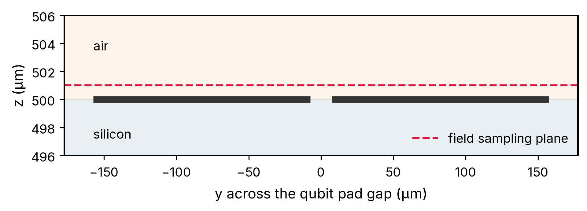
Palace saved the first two eigenfields under output/palace/paraview/eigenmode/Cycle00000{1,2}/data.pvtu. The images sample their electric-field magnitude 1 µm above the metal plane at model coordinate \(z=501\) µm. The qubit view zooms in on the pads; the readout view shows the full meander. Palace’s visualization guide explains that the tangential field is continuous across tetrahedra but the normal component can jump, leaving triangular seams in a planar cut. We clip the low values and smooth the display over 0.4 µm near the pads and 1.0 µm across the meander. Frequencies and participations use the unsmoothed solver data. Gray lies outside the solved domain, and eigenmode amplitudes have arbitrary normalization. The images are saved in the notebook; the cross-section below marks the sampling plane.

fig, ax = plt.subplots(figsize=(6.5, 2.4))
ax.axhspan(496, 500, color="steelblue", alpha=0.12)
ax.axhspan(500, 506, color="darkorange", alpha=0.08)
pad_outer = QUBIT_PAD_SIZE[0] + QUBIT_PAD_GAP / 2
ax.hlines(
    [500, 500],
    [-pad_outer, QUBIT_PAD_GAP / 2],
    [-QUBIT_PAD_GAP / 2, pad_outer],
    color="0.2",
    linewidth=5,
)
ax.axhline(501, color="crimson", linestyle="--", label="field sampling plane")
ax.text(-pad_outer, 497.2, "silicon")
ax.text(-pad_outer, 503.5, "air")
ax.set_xlim(-pad_outer - 20, pad_outer + 20)
ax.set_ylim(496, 506)
ax.set_xlabel("y across the qubit pad gap (µm)")
ax.set_ylabel("z (µm)")
ax.grid(False)
ax.legend(loc="lower right")
fig.tight_layout()
plt.show()
plt.close(fig)

../_images/45a2270f85341e6291e647933b67ec1915532ee8a216c87cfb460431f07a0c2f.png

field_root = Path("sim_palace_qubit_resonator/output/palace/paraview/eigenmode")


def _plot_eigenfield(mode: int, extent: tuple[float, float, float, float]) -> None:
    pv = importlib.import_module("pyvista")

    samples = 700 if extent[1] - extent[0] < 500 else 1000
    x = np.linspace(extent[0], extent[1], samples)
    y = np.linspace(extent[2], extent[3], samples)
    grid_x, grid_y = np.meshgrid(x, y)
    points = np.column_stack((
        grid_x.ravel(),
        grid_y.ravel(),
        np.full(grid_x.size, 501.0),
    ))
    path = field_root / f"Cycle{mode:06d}" / "data.pvtu"
    sampled = pv.PolyData(points).sample(pv.read(path))
    valid = np.asarray(sampled.point_data["vtkValidPointMask"], dtype=bool).reshape(
        grid_x.shape
    )
    e_real = np.asarray(sampled.point_data["E_real"], dtype=float)
    e_imag = np.asarray(sampled.point_data["E_imag"], dtype=float)
    magnitude = np.sqrt(np.sum(e_real**2 + e_imag**2, axis=1)).reshape(grid_x.shape)
    positive = magnitude[valid & (magnitude > 0)]
    vmax = float(np.percentile(positive, 99.5))
    vmin = max(vmax / 150, float(np.percentile(positive, 25)))
    sigma_um = 0.4 if x[-1] - x[0] < 500 else 1.0
    sigma = (sigma_um / (y[1] - y[0]), sigma_um / (x[1] - x[0]))
    log_field = np.log(np.where(valid, np.maximum(magnitude, vmin), vmin))
    weight = valid.astype(float)
    smooth_weight = gaussian_filter(weight, sigma)
    shown = np.where(
        valid,
        np.exp(
            gaussian_filter(log_field * weight, sigma)
            / np.maximum(smooth_weight, 1e-12)
        ),
        np.nan,
    )
    cmap = plt.get_cmap("magma").copy()
    cmap.set_bad("0.94")

    fig, ax = plt.subplots(figsize=(6.5, 5.6))
    image = ax.imshow(
        shown,
        origin="lower",
        extent=extent,
        cmap=cmap,
        norm=LogNorm(vmin=vmin, vmax=vmax),
        interpolation="none",
    )
    ax.set_aspect("equal")
    ax.grid(False)
    ax.set_xlabel("x (µm)")
    ax.set_ylabel("y (µm)")
    ax.set_title(f"Mode {mode}: {eig_f_re[mode - 1]:.3f} GHz")
    fig.colorbar(image, ax=ax, label=r"$|\mathbf{E}|$ (V/m)")
    plt.show()
    plt.close(fig)


if field_root.exists():
    _plot_eigenfield(int(eig_m[i_qubit]), (-230, 230, -250, 250))
    bounds = component.dbbox()
    _plot_eigenfield(
        int(eig_m[i_res]), (bounds.left, bounds.right, bounds.bottom, bounds.top)
    )
else:
    logger.info("Palace field files are needed to regenerate the embedded plots")

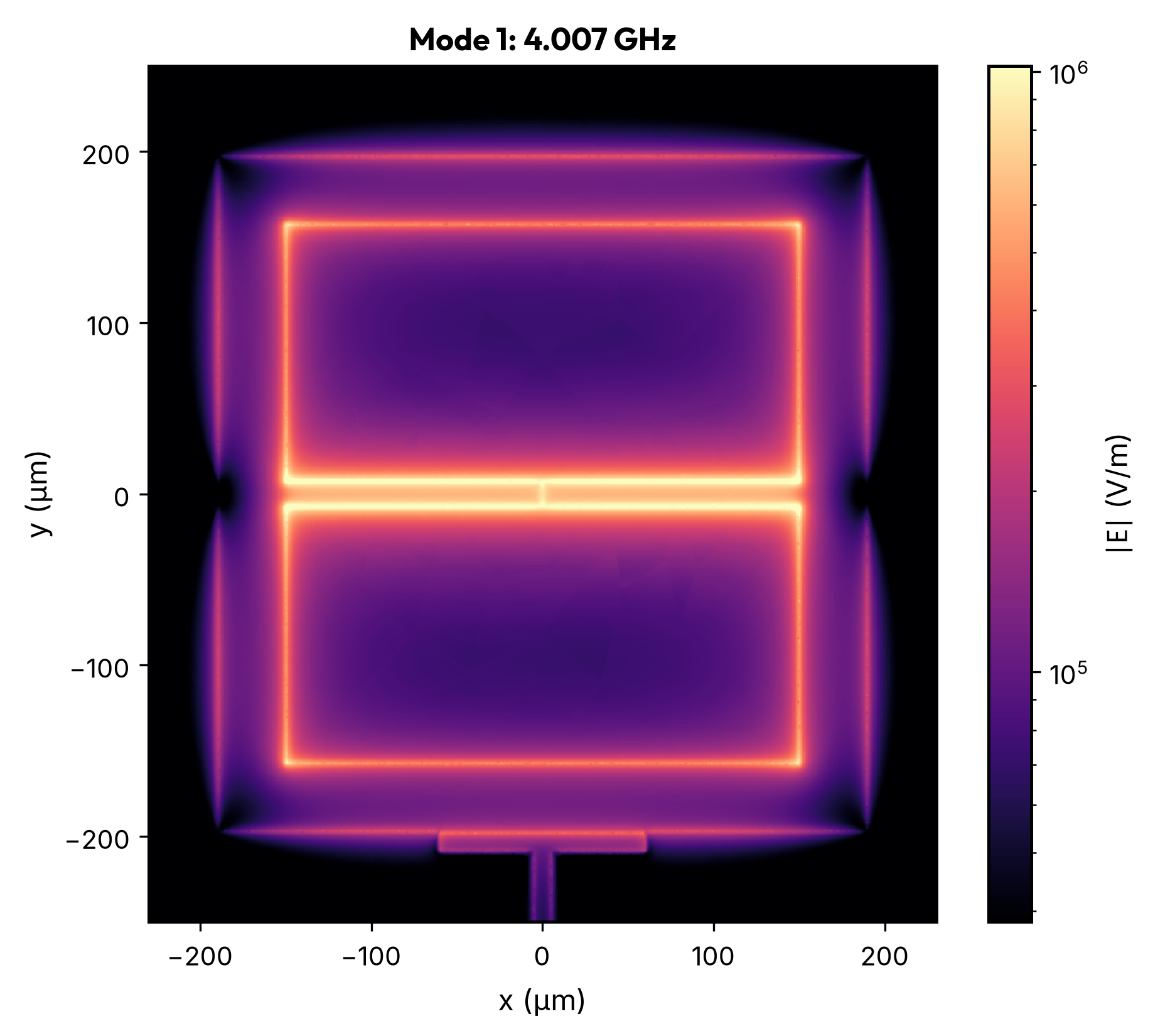
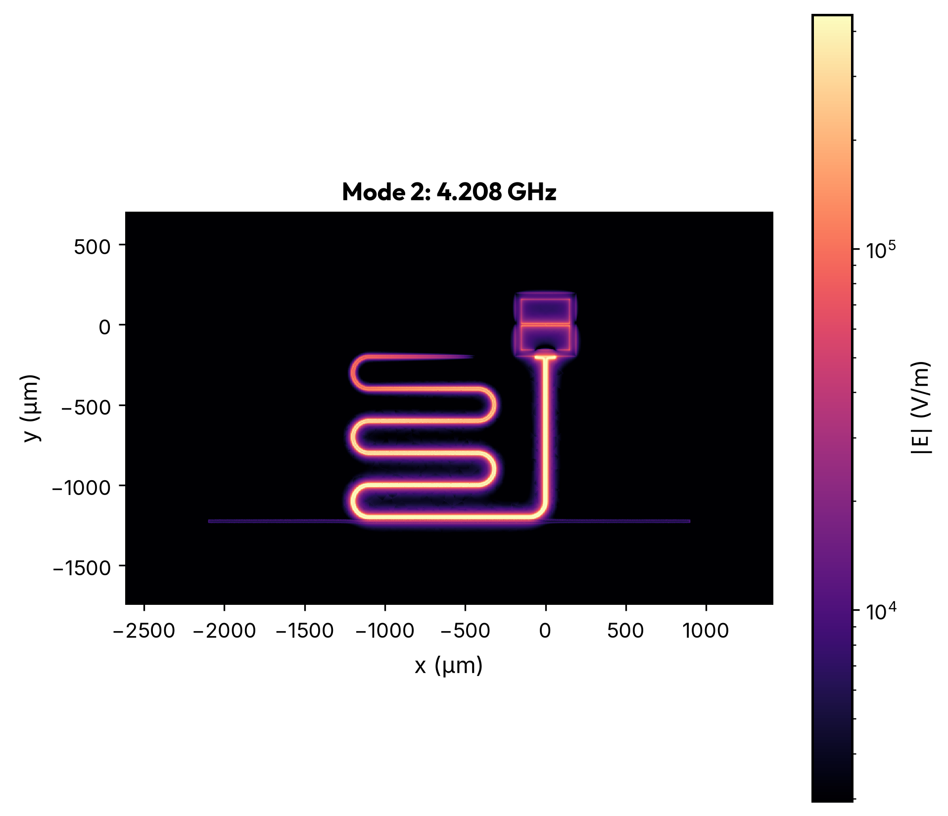
../_images/e5e0c19eb9095367e9aebb781d0fbdc71e93c264495bbeb4daf0bee3408d7d33.png

../_images/a80486f0ef39abac6f6c619e87c0d4d6d76d5dca1b444bb8afb6ce90f160f254.png

The qubit-like mode concentrates field across the pad gap and along the pad edges. Complex \(E_z\) probes above the two pad interiors are 180 degrees out of phase in this mode, consistent with a differential pad excitation. The readout mode follows the meander as a quarter-wave standing wave. Their small detuning leaves some field on both parts of the layout, consistent with the nonzero junction and feed-port participation of each mode.

Summary#

A qpdk layout goes to a full-wave eigenmode spectrum with no commercial solver license. With larger qubit pads, a longer probeline and a larger domain, retuning the junction inductance retains a nearby qubit/readout pair. Junction participation, feed-port coupling and the saved electric fields distinguish the two. The CPW estimate gives a starting length; the Palace solve checks the adjusted layout.

The SAX circuit models in QPDK Models and Circuit Simulation with QPDK miss the geometry-dependent effects captured here (fringing, loading, meander parasitics) but cost almost nothing, so the two complement each other: circuit models to explore, FEM to verify and calibrate. The next step, extracting the Hamiltonian, anharmonicities and dispersive couplings from these eigenmodes via energy participation [MLM+21, NPV+12], is what tools such as pyEPR do.

References#

[CFL+22]

M. Checchin, D. Frolov, A. Lunin, A. Grassellino, and A. Romanenko. Measurement of the Low-Temperature Loss Tangent of High-Resistivity Silicon Using a High- Q Superconducting Resonator. Physical Review Applied, 18(3):034013, September 2022. doi:10.1103/PhysRevApplied.18.034013.

[KYG+07]

Jens Koch, Terri M. Yu, Jay Gambetta, A. A. Houck, D. I. Schuster, J. Majer, Alexandre Blais, M. H. Devoret, S. M. Girvin, and R. J. Schoelkopf. Charge-insensitive qubit design derived from the Cooper pair box. Physical Review A, 76(4):042319, October 2007. doi:10.1103/PhysRevA.76.042319.

[KKY+19]

P. Krantz, M. Kjaergaard, F. Yan, T. P. Orlando, S. Gustavsson, and W. D. Oliver. A quantum engineer's guide to superconducting qubits. Applied Physics Reviews, 6(2):021318, June 2019. doi:10.1063/1.5089550.

[MP12]

David M. Pozar. Microwave Engineering. John Wiley & Sons, Inc., 4 edition, 2012. ISBN 978-0-470-63155-3.

[MLM+21] (1,2,3,4,5)

Zlatko K. Minev, Zaki Leghtas, Shantanu O. Mundhada, Lysander Christakis, Ioan M. Pop, and Michel H. Devoret. Energy-participation quantization of Josephson circuits. npj Quantum Information, 7(1):131, September 2021. doi:10.1038/s41534-021-00461-8.

[NPV+12] (1,2,3)

S. E. Nigg, H. Paik, B. Vlastakis, G. Kirchmair, S. Shankar, L. Frunzio, M. H. Devoret, R. J. Schoelkopf, and S. M. Girvin. Black-box superconducting circuit quantization. Physical Review Letters, 108(24):240502, June 2012. doi:10.1103/PhysRevLett.108.240502.

[Sim01]

Rainee Simons. Coplanar Waveguide Circuits, Components, and Systems. Number v. 165 in Wiley Series in Microwave and Optical Engineering. Wiley Interscience, New York, 2001. ISBN 978-0-471-46393-1. doi:10.1002/0471224758.