Getting started with Palace
This page takes you from a gdsfactory component to S-parameters with gsim.palace. You build the
geometry, stack, ports and mesh on your own machine, look at the mesh, solve on GDSFactory+ cloud, and read the result
as a SParams object or a Touchstone file. The last section shows how to run the same inputs on a Palace you run
yourself.
The example is a 300 µm coplanar waveguide (CPW) in the generic PDK, so everything below runs without a foundry PDK. The same steps are used by the CPW tutorial, which runs an 800 µm line in the open IHP PDK and shows the results of its cloud run.
What you need
- Python 3.12. gsim declares
requires-python = "~=3.12.0". pip install gsim. This brings in gdsfactory (with its generic PDK,gf.gpdk), the Gmsh mesher and thegdsfactoryplusclient that submits cloud jobs. You do not need a local Palace installation for the cloud route.- A GDSFactory+ account, for the cloud solve in step 5. Everything before
run()works without one.
For the IHP open PDK used by the tutorial notebooks, also install ihp-gdsfactory.
1. A component
Palace needs the metal geometry and one gdsfactory port per electrical port. Put the port at the centre of the signal
conductor, on the conductor's layer, with the signal width, and mark it port_type="electrical".
import gdsfactory as gf

from gsim.palace import DrivenSim

gf.gpdk.PDK.activate()


@gf.cell
def gsg_line(length=300, s_width=10, g_width=40, gap_width=6, layer=gf.gpdk.LAYER.M1):
    """Ground-signal-ground line with one port at each end of the signal."""
    c = gf.Component()
    ground_top = c << gf.c.rectangle((length, g_width), centered=True, layer=layer)
    ground_top.move((0, (g_width + s_width) / 2 + gap_width))
    c << gf.c.rectangle((length, s_width), centered=True, layer=layer)
    ground_bottom = c << gf.c.rectangle((length, g_width), centered=True, layer=layer)
    ground_bottom.move((0, -(g_width + s_width) / 2 - gap_width))
    for name, x, orientation in (("o1", -length / 2, 180), ("o2", length / 2, 0)):
        c.add_port(name=name, center=(x, 0), width=s_width, orientation=orientation, port_type="electrical", layer=layer)
    return c
2. Stack and airbox
set_stack() reads the layer stack of the active PDK, here the generic one. set_airbox() pads the model with air.
All lengths are in µm.
sim = DrivenSim()
sim.set_output_dir("./palace-gsg-line")
sim.set_geometry(gsg_line())
sim.set_stack(substrate_thickness=2.0)
sim.set_airbox(margin_x=0, margin_y=50.0, z_above=100.0, z_below=100.0)
substrate_thicknessis the depth belowz=0of the oxide fill. By default the PDK's own silicon substrate layer is left out of the model (include_substrate=False), and gsim logs a warning saying so when the PDK has one. Passinclude_substrate=Trueto mesh it as lossy silicon. To take the PDK's layer stack verbatim, as the IHP notebooks do, useset_stack(pdk_authoritative=True).set_airbox()addsmargin_xandmargin_yaround the layout andz_aboveandz_belowabove and below the stack. Heremargin_x=0keeps the domain ends flush with the ends of the line, where the ports sit: the example's mesh spans x = ±150 µm, the length of the line, and y = ±101 µm, the 51 µm half-width of the three conductors plus the 50 µm margin.- Without an airbox the outer boundary would touch the dielectric directly, and gsim warns about it when you mesh. The outer wall of a driven model with lumped ports is absorbing by default.
3. Ports
Lumped CPW ports, one per end of the line:
for port in ("o1", "o2"):
    sim.add_cpw_port(port, layer="metal1", s_width=10, gap_width=6, length=5.0)
sim.set_driven(fmin=1e9, fmax=100e9, num_points=40)
print(sim.validate_config())
add_cpw_port takes the layout's signal width and gap width and builds two lumped elements, one in each gap, driven
with opposite sign to excite the coplanar mode. length is the port's extent along the line, offset shifts it
inwards (it defaults to length / 2, which puts the port flush with the conductor end), and impedance is the
reference impedance, 50 Ω by default. Every port is excited in turn, so a two-port model gives the full S-matrix.
set_driven() sets the frequency sweep, and validate_config() lists configuration errors before you spend time
on meshing.
A wave port instead solves the actual 2D mode of the port face. It replaces add_cpw_port like this:
wave = DrivenSim()
wave.set_output_dir("./palace-gsg-line-wave")
wave.set_geometry(gsg_line())
wave.set_stack(substrate_thickness=2.0)
wave.set_airbox(margin_x=0, margin_y=50.0, z_above=100.0, z_below=100.0)
for port in ("o1", "o2"):
    wave.add_wave_port(port, layer="metal1", max_size=True)
wave.set_driven(fmin=1e9, fmax=100e9, num_points=40)
max_size=True makes the port face fill the airbox boundary on that side. With wave ports, gsim makes the outer wall PEC
instead of absorbing, because Palace solves the port mode with PEC outer edges; see
Numeric wave-port boundaries for the rule and for absorbing_boundary=True.
The wave-port version of this example is a larger model (10,362 tetrahedra at the coarse preset, against 7,897 for the
lumped one; see step 4). To compare both port types on a real line, see the
lumped-port and wave-port tutorials, and for multimode and
terminal ports see Terminal wave ports.
4. Mesh, and look at it
result = sim.mesh(preset="coarse")
print(result.mesh_stats["tetrahedra"])
print(result.mesh_stats["field_dofs"]["estimated_field_dofs"])
sim.plot_mesh(show_groups=["metal", "P"])
mesh() writes palace.msh and metadata.json (the sizing counts) to the output directory; the Palace configuration
comes later, from write_config() or run(). The three presets set the element size near conductors
(refined_mesh_size) and in the bulk (max_mesh_size), both in µm. Pass either as a keyword to override the preset.
The counts below are for this example with lumped ports, measured with gsim 0.9.0; a different Gmsh version can change
them slightly.
| Preset | refined_mesh_size |
max_mesh_size |
Tetrahedra | Estimated field DOFs (order 2) |
|---|---|---|---|---|
"coarse" |
10 | 600 | 7,897 | 50,992 |
"default" |
5 | 300 | 20,220 | 129,804 |
"fine" |
2 | 70 | 55,061 | 353,272 |
Use coarse to check that the geometry, ports and boundaries are what you meant. It is not meant for results. On this
example coarse and default both log Small conductor feature detected (6.000 um) may be under-resolved by
refined_mesh_size=..., because the gaps are 6 µm wide and the heuristic asks for elements of at most 3 µm; fine does
not log it. The warning is a heuristic, and a mesh without it is not thereby converged: compare two meshes before you
trust a number (see Mesh).
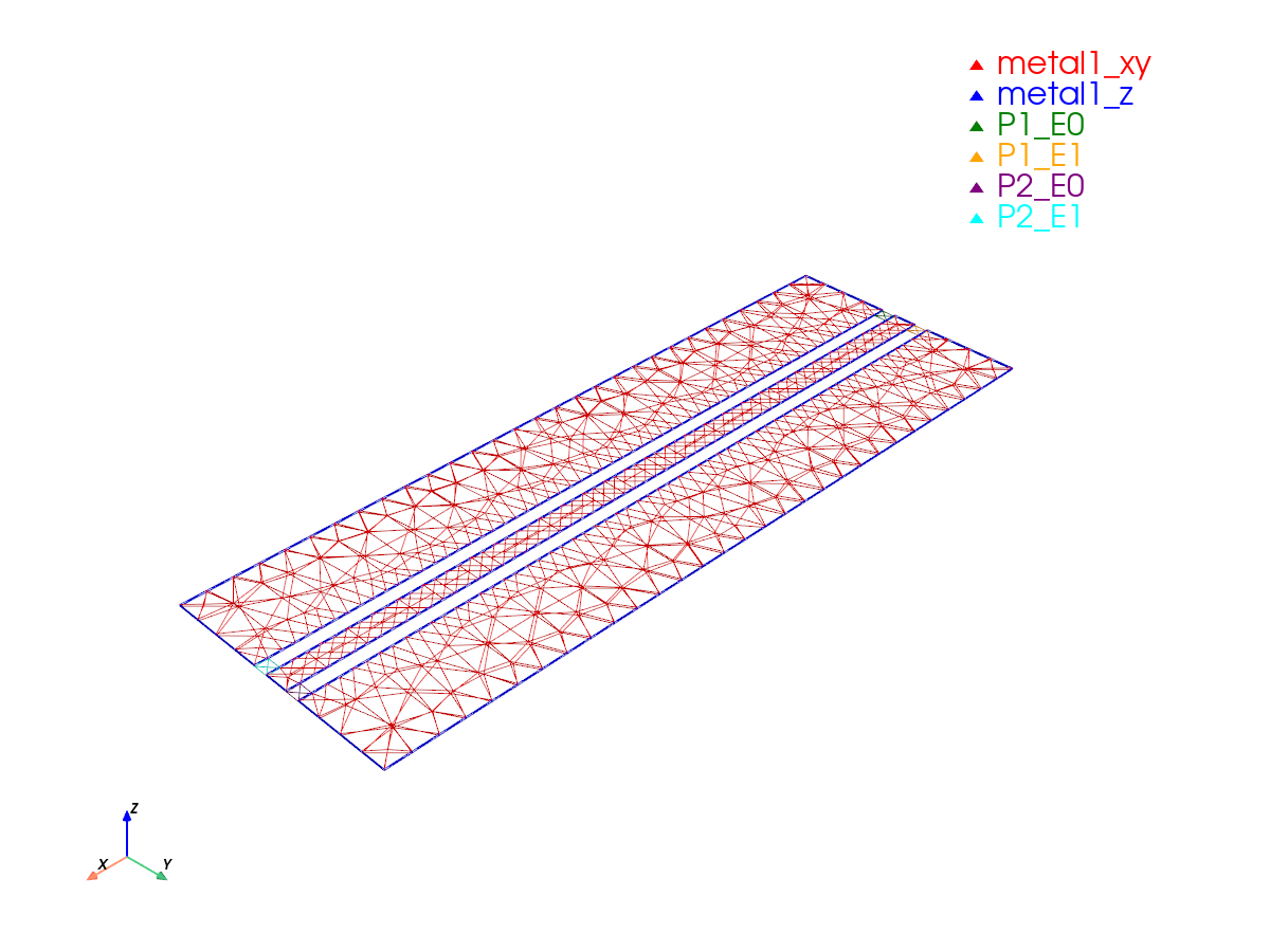
The coarse mesh, drawn with show_groups=["metal", "P"]: the metal1 surfaces and the port sheets P1_E0, P1_E1,
P2_E0, P2_E1, one pair of sheets per port. plot_mesh() writes a PNG to mesh.png in the output directory; pass
interactive=True to open a 3D view.
The estimated field DOFs are what the cloud uses to size the job, together with the tetrahedron count. Read them before you submit: see Cloud sizing metadata.
5. Run on the cloud
run() writes config.json from the current settings, uploads the mesh and configuration, starts the job, waits for
it, downloads the results into sim-data-<job name>/ in the current directory and parses them into a SParams object.
So after mesh() you do not have to call write_config() yourself; call it if you want to inspect the configuration
before submitting.
check_cache=True first looks for a finished job whose inputs are byte-identical to yours and reuses its results
instead of starting a new one; when none matches, a new job starts. See Result caching.
If a job is rejected as too large, or fails with exit code 137 (SIGKILL, often out of memory), coarsen the mesh or shrink the model; see Palace size limits and out-of-memory failures.
6. Read the results
SParams indexes by port-name pair as results["to", "from"], and s11, s21, s12, s22 are shorthand on a
two-port model. Frequencies are in GHz.
results.freq  # GHz
results.s21.db  # |S21| in dB
results["o2", "o1"].deg  # phase of S(o2, o1) in degrees

results.plot()  # matplotlib: magnitude and phase
results.plot_interactive()  # plotly, toggle traces in the legend

network = results.to_skrf()  # scikit-rf Network, frequency in Hz
network.plot_s_db(1, 0)  # |S21| in dB
results.write_touchstone("gsg_line")  # gsg_line.s2p
write_touchstone() adds the .s2p suffix when the name has none and writes frequencies in Hz with the port names in
! Port[i] comments. save_npz() and SParams.from_file() store and reload the same data without Touchstone's
text format. For length sweeps, de-embedding and RLGC extraction with scikit-rf, see
Transmission-line analysis.
7. Check the run
A job that finished is not a result you can trust yet. gsim reads the solver log and the run metadata and reports convergence, adaptive-sweep and port-mode checks separately: see Palace: Checking a Run.
Run Palace locally
run_local() solves the same mesh and config.json on your own machine, with a Palace you run yourself. It returns
the same SParams object as the cloud run for a driven simulation.
sim.mesh(preset="default")
sim.write_config()  # run_local() does not write config.json; run() does
results = sim.run_local(log_path="palace.log")
run_local() needs mesh() and write_config() first. Without config.json it raises FileNotFoundError and tells you
to call write_config(). What you call again after a change depends on what you changed:
- Solver settings (for example the frequency sweep from
set_driven()): callwrite_config()again. - Geometry, stack or airbox, or ports (including a port's
impedance,lengthoroffset): callmesh()again, thenwrite_config().mesh()captures the mesh and the ports, andwrite_config()writesconfig.jsonfrom that capture, sowrite_config()alone keeps the old mesh and the old port values.
Palace writes its tables to <output directory>/output/palace/ (palace is the default model_name of mesh()).
log_path keeps the solver log even when the run fails; hand its text to
validate_solution as in step 7.
Which Palace runs
run_local() takes the first of these that exists:
- The
palace_executable=argument. - The
PALACE_EXECUTABLEenvironment variable. bin/palaceunder the current directory, the output directory or its parent.- With
use_apptainer=True(it defaults toFalse) and none of the above: an Apptainer image, frompalace_sif_path=,PALACE_SIFor aPalace.sifin those same places. - Otherwise the first Palace that gsim finds:
PALACE_BIN, thenpalaceonPATH, then gsim's own cached runtime and, if there is none, a download of it. (A runtime from an installedpalace-toolkitpackage comes after those.)
The download is the part that is easy to trip over:
- It exists only for Linux on x86_64. It fetches a prebuilt CPU runtime of Palace 0.18.0 from the PalaceToolkit
project's GitHub releases the first time you need it and caches it under
~/.cache/palacetoolkit/runtime.PALACETOOLKIT_RUNTIME_DIRmoves the cache,PALACETOOLKIT_AUTO_DOWNLOAD_BINARY=0turns the download off andPALACETOOLKIT_PALACE_CPU_TAGnames another release tag. - On Windows and macOS gsim downloads nothing. With no Palace found,
run_local()raises aFileNotFoundErrorthat starts "Palace executable not found", as it does on a Windows machine with nothing installed. - On Windows, use WSL2: install gsim in a Python 3.12 environment inside a WSL2 Linux distribution and run your script there. On an x86_64 distribution that is the Linux x86_64 path, with the download above. The authors have not run these WSL2 steps; the code path is the one any Linux x86_64 machine takes.
- Windows on ARM normally runs an aarch64 WSL2 distribution. There
platform.machine()isaarch64, gsim's check for Linux on x86_64 (_is_linux_x86_64()ingsim/palace/runtime.py) fails and nothing is downloaded. Install or build Palace yourself and pointpalace_executable=orPALACE_EXECUTABLEat it, as in the next item. Rununame -min the distribution to see which you have. - To use a Palace you built or installed, pass
palace_executable=or setPALACE_EXECUTABLE. gsim starts it aspalace -np <ranks> [-nt <threads>] config.json, so it must accept the Palace launcher's arguments.
The number of MPI ranks is chosen from the problem size: at most 4 for a 3D model, fewer for a small one, and one rank
with OpenMP threads for a 2D cross-section. Pass num_processes= or num_threads= to override it; gsim warns when you
ask for more ranks than the direct solver can use on a problem of that size.
Local and cloud runs differ
Crackon conductors. For a 3D model gsim writes"Crack": trueon everyBoundaries.Conductivityentry inconfig.json, so that Palace 0.19 and later keeps the conductor as a thick conductor instead of reading its boundary as a thin film. Palace 0.18 rejects the key and always treats such a boundary as cracked, so the model is the same without it. When the Palace thatrun_local()starts is known to be older than 0.19, it gets a temporary copy of the configuration without the key, which is deleted after the run.config.jsonkeeps the key, and so does what you upload to the cloud. gsim knows the version of its own runtime; for a Palace you installed it askspalace --version, and if the answer is not a release number such asv0.18.0it keeps the key and leaves Palace to accept or reject it.- Palace version. The auto-downloaded runtime is Palace 0.18.0, and the cloud runs a different build, a specific Palace commit. The difference documented so far is the line integration behind voltage and impedance paths: the local 0.18.0 runtime samples the path with its default count of 100 and does not gain the element-wise integration of the cloud runtime (see Boundary-mode path integration). Compare a local and a cloud run of the same model before you combine them in one study.
Next steps
- CPW tutorial, lumped ports: this page's steps on an 800 µm IHP line, 300 frequency points from 1 to 100 GHz.
- CPW tutorial, wave ports: the same line with wave ports.
- Microstrip and branch-line coupler: other layouts.
- Width sweep: several simulations in parallel.
- Length sweep and de-embedding: extract line parameters from lumped- and wave-port runs.
- Palace guide: solver settings, mesh options and result handling.
- Cloud guide: sizing, caching and failed jobs.