Ring filter

Calculations

For a ring resonator we need to define:

Optical parameters:

• coupling coefficient: will define resonance extinction ratio for a particular ring loss.

• Free spectral range.

Electrical parameters:

• VpiL

• Resistance

import gdsfactory as gf
import numpy as np


def ring(
    wl: np.ndarray,
    wl0: float,
    neff: float,
    ng: float,
    ring_length: float,
    coupling: float,
    loss: float,
) -> np.ndarray:
    """Returns Frequency Domain Response of an all pass filter.

    Args:
        wl: wavelength in  um.
        wl0: center wavelength at which neff and ng are defined.
        neff: effective index.
        ng: group index.
        ring_length: in um.
        loss: dB/um.
    """
    transmission = 1 - coupling
    neff_wl = (
        neff + (wl0 - wl) * (ng - neff) / wl0
    )  # we expect a linear behavior with respect to wavelength
    out = np.sqrt(transmission) - 10 ** (-loss * ring_length / 20.0) * np.exp(
        2j * np.pi * neff_wl * ring_length / wl
    )
    out /= 1 - np.sqrt(transmission) * 10 ** (-loss * ring_length / 20.0) * np.exp(
        2j * np.pi * neff_wl * ring_length / wl
    )
    return abs(out) ** 2


if __name__ == "__main__":
    import matplotlib.pyplot as plt

    loss = 0.03  # [dB/μm] (alpha) waveguide loss
    neff = 2.46  # Effective index of the waveguides
    wl0 = 1.55  # [μm] the wavelength at which neff and ng are defined
    radius = 5
    ring_length = 2 * np.pi * radius  # [μm] Length of the ring
    coupling = 0.5  # [] coupling of the coupler
    wl = np.linspace(1.5, 1.6, 1000)  # [μm] Wavelengths to sweep over
    wl = np.linspace(1.55, 1.60, 1000)  # [μm] Wavelengths to sweep over
    ngs = [4.182551, 4.169563, 4.172917]
    thicknesses = [210, 220, 230]

    # widths = np.array([0.4, 0.45, 0.5, 0.55, 0.6])
    # ngs = np.array([4.38215238, 4.27254985, 4.16956338, 4.13283219, 4.05791982])

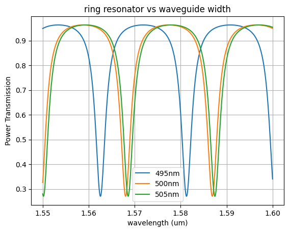
    widths = np.array([0.495, 0.5, 0.505])
    neffs = np.array([2.40197253, 2.46586378, 2.46731758])
    ng = 4.2  # Group index of the waveguides

    for width, neff in zip(widths, neffs):
        p = ring(
            wl=wl,
            wl0=wl0,
            neff=neff,
            ng=ng,
            ring_length=ring_length,
            coupling=coupling,
            loss=loss,
        )
        plt.plot(wl, p, label=f"{int(width*1e3)}nm")

    plt.title("ring resonator vs waveguide width")
    plt.xlabel("wavelength (um)")
    plt.ylabel("Power Transmission")
    plt.grid()
    plt.legend()
    plt.show()

Layout

gdsfactory easily enables you to layout Component with as many levels of hierarchy as you need.

A Component is a canvas where we can add polygons, references to other components or ports.

Lets add two references in a component.

import gdsfactory as gf
import toolz

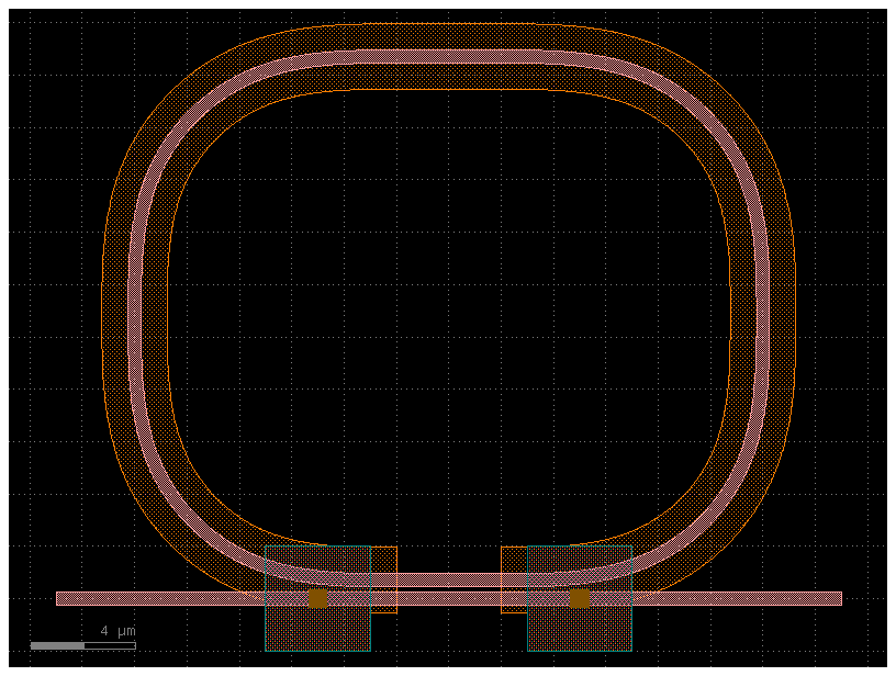
c = gf.components.ring_single_heater(gap=0.2, radius=10, length_x=4)
c.plot()

scene = c.to_3d()
scene.show()

Lets define a ring function that also accepts other component specs for the subcomponents (straight, coupler, bend)

xs = gf.cross_section.metal3(width=5)

ring = gf.components.ring_single_heater(gap=0.2, radius=10, length_x=4)
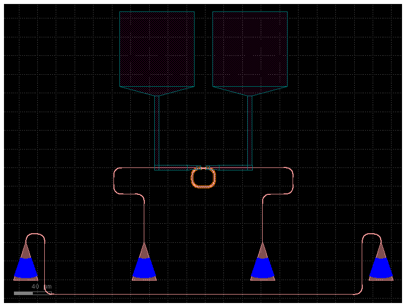
ring_with_pads = gf.routing.add_pads_top(
    ring,
    port_names=["r_e3", "l_e1"],
    cross_section=xs,
    fanout_length=100,
)
ring_with_pads_grating_couplers = gf.routing.add_fiber_array(
    ring_with_pads, with_loopback=True
)
ring_with_pads_grating_couplers.show()
ring_with_pads_grating_couplers.plot()

/home/runner/micromamba/lib/python3.11/site-packages/gdsfactory/pdk.py:425: UserWarning: {'width': 5.0} are ignored for cross_section 'xs_d27ce971'
  warnings.warn(

ring = gf.components.ring_single_heater(gap=0.2, radius=10, length_x=4)
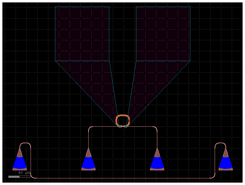
ring_with_grating_couplers = gf.routing.add_fiber_array(ring, with_loopback=True)
c = gf.routing.add_electrical_pads_top(
    ring_with_grating_couplers, port_names=("l_e1", "r_e3")
)
c.plot()