Instances and ports

Gdsfactory defines your component once in memory and can add multiple Instances (references) to the same component.

As you build components, you can include references to other components. Adding an instance is like having a pointer to a component.

The GDSII specification allows the use of instances, and similarly gdsfactory uses them (with the add_ref() function). what is an instance? Simply put: An instance does not contain any geometry. It only points to an existing geometry.

Say you have a ridiculously large polygon with 100 billion vertices that you call BigPolygon. It is huge, and you need to use it in your design 250 times. Well, a single copy of BigPolygon takes up 1MB of memory, so you do not want to make 250 copies of it You can instead instantiate the polygon 250 times. Each instance only uses a few bytes of memory – it only needs to know the memory address of BigPolygon, position, rotation and mirror. This way, you can keep one copy of BigPolygon and use it again and again.

You can start by making a blank Component and add a single polygon to it.

import gdsfactory as gf

# Create a blank Component
p = gf.Component()

# Add a polygon.
xpts = [0, 0, 5, 6, 9, 12]
ypts = [0, 1, 1, 2, 2, 0]
# The zip function takes two lists (xpts and ypts) and pairs their elements together. 
# The first element of xpts is paired with the first of ypts, the second with the second, and so on.
# This creates a sequence of (x, y) tuples. A tuple is a data structure that consists of multiple parts.
# list(...): The output of zip is converted into a list of these coordinate tuples.
p.add_polygon(list(zip(xpts, ypts)), layer=(2, 0))

# Plot the Component with the polygon in it.
p.plot()

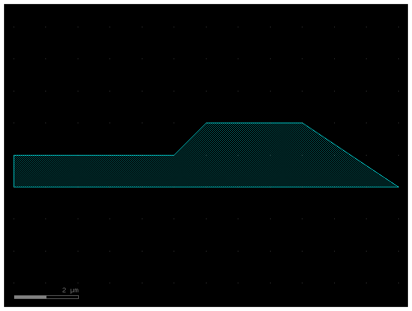
Now, you want to reuse this polygon repeatedly without creating multiple copies of it.

To do so, you need to make a second blank Component, this time called c.

In this new Component you instantiate our Component p which contains our polygon.

c = gf.Component()  # Create a new blank component.
poly_ref = c.add_ref(p)  # instantiate the component "p" that has the polygon in it.
c.plot()

You just made a copy of your polygon – but remember, you did not actually make a second polygon, you just made a reference (aka pointer) to the original polygon. Let us add two more references to c:

poly_ref2 = c.add_ref(p) 
poly_ref3 = c.add_ref(p)  
c.plot()

Now you have 3x polygons all on top of each other. Again, this would appear useless, except that you can manipulate each instance independently. Notice that when you called c.add_ref(p) above, we saved the result to a new variable each time (poly_ref, poly_ref2, and poly_ref3)? You can use those variables to reposition the instances.

poly_ref2.rotate(90)  # Rotate the 2nd instance we made by 90 degrees.
poly_ref3.rotate(180)  # Rotate the 3rd instance we made by 180 degrees.
c.plot()

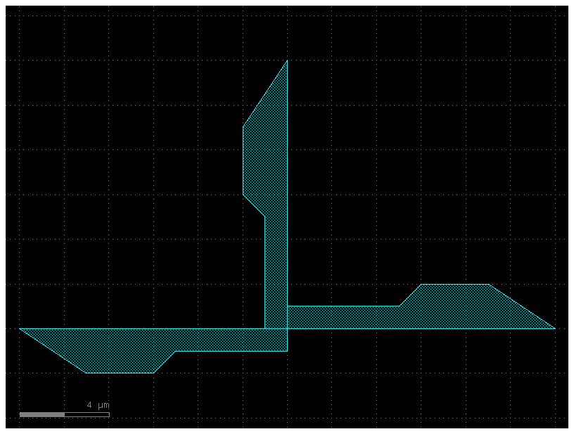
Now you are getting somewhere! You have only had to make the polygon once, but you are able to reuse it as many times as you want.

Modifying the instance

What happens when you change the original geometry that the reference points to? In your case, your references in c all point to the Component p that with the original polygon. Let us try adding a second polygon to p.

First you add the second polygon and make sure P looks like you expect:

# Add a 2nd polygon to "p".
xpts = [14, 14, 16, 16]
ypts = [0, 2, 2, 0]
p.add_polygon(list(zip(xpts, ypts)), layer=(1, 0))
p

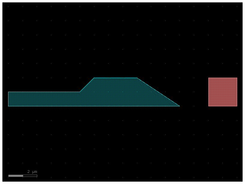
That looks good. Now let us find out what happened to c that contains the three references. Keep in mind that you have not modified c or executed any functions/operations on c – all you have done is modify p.

c.plot()

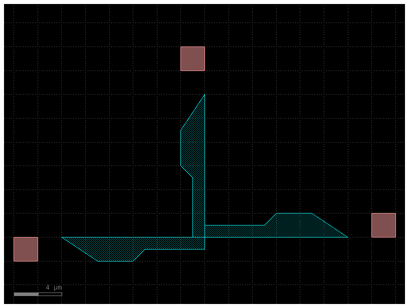
When you modify the original geometry, all of the references automatically reflect the modifications. This is very powerful, because you can use this to make very complicated designs from relatively simple elements in a computation- and memory-efficient way.

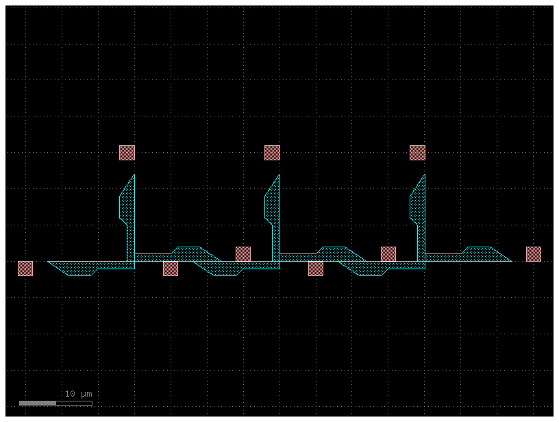
Let us try making references a level deeper by referencing c. Note here we use the << operator to add the references – this is just shorthand, and is exactly equivalent to using add_ref()

c2 = gf.Component()
d_ref1 = c2.add_ref(c)  # Reference the Component "c" that 3 references in it.
d_ref2 = c2 << c  # Use the "<<" operator to create a 2nd reference to c.plot().
d_ref3 = c2 << c 

d_ref1.move((20, 0))
d_ref2.move((40, 0))

c2

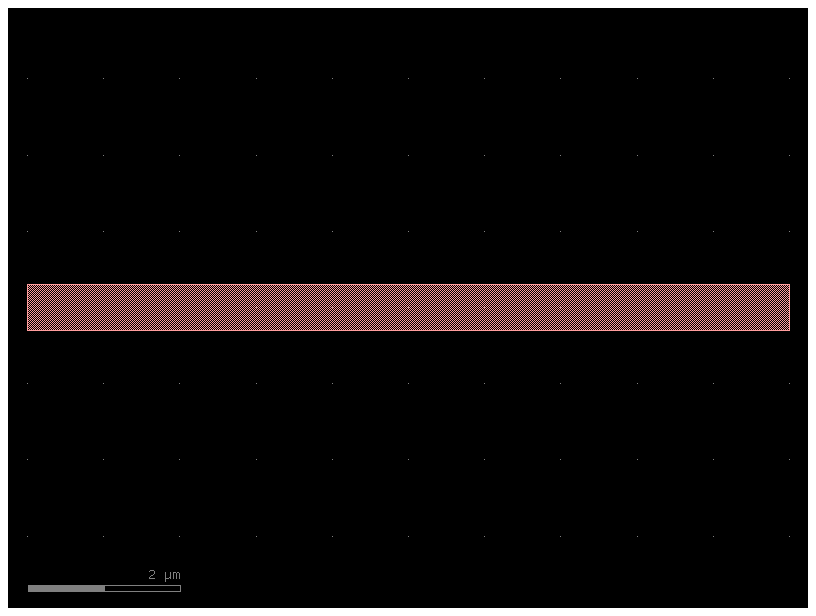
As you have seen you have two ways to add a reference to our component:

1. Create the reference and add it to the component

c = gf.Component()
wr = c.add_ref(gf.components.straight(width=0.6))
c.plot()

2. Or do it in a single line

c = gf.Component()
wr = c << gf.components.straight(width=0.6)
c.plot()

In both cases you can move the reference wr after created

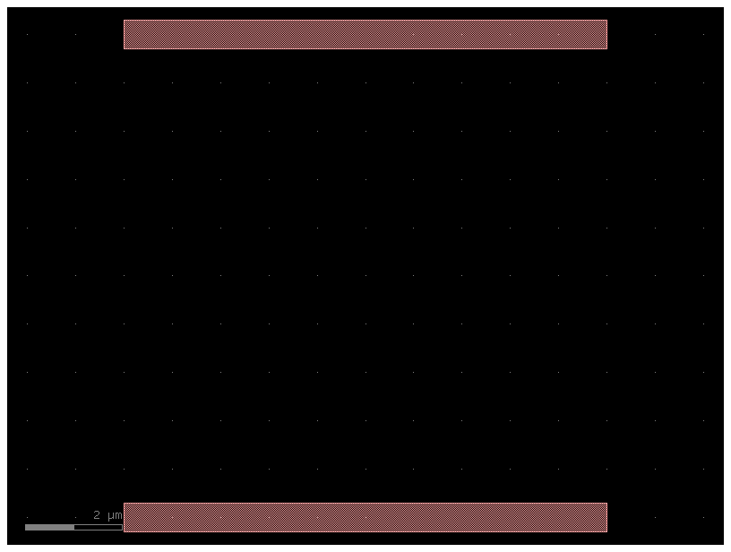
c = gf.Component()
wr1 = c << gf.components.straight(width=0.6)
wr2 = c << gf.components.straight(width=0.6)
wr2.movey(10)

# This takes the ports from the bottom waveguide (wr1), which are named o1 and o2, and adds them to c with the prefix "bot_".
# The new ports on c will be named bot_o1 and bot_o2.
c.add_ports(wr1.ports, prefix="bot_")

# This does the same for the upper waveguide (wr2), creating 2 new ports on c named top_o1 and top_o2.
c.add_ports(wr2.ports, prefix="top_")

c.pprint_ports()

┏━━━━━━━━┳━━━━━━━┳━━━━━━━━━━━━━┳━━━━━━━━━━┳━━━━━━━━━━━━━━┳━━━━━━━━━━━┓
┃ name   ┃ width ┃ orientation ┃ layer    ┃ center       ┃ port_type ┃
┡━━━━━━━━╇━━━━━━━╇━━━━━━━━━━━━━╇━━━━━━━━━━╇━━━━━━━━━━━━━━╇━━━━━━━━━━━┩
│ bot_o1 │ 0.6   │ 180.0       │ WG (1/0) │ (0.0, 0.0)   │ optical   │
│ bot_o2 │ 0.6   │ 0.0         │ WG (1/0) │ (10.0, 0.0)  │ optical   │
│ top_o1 │ 0.6   │ 180.0       │ WG (1/0) │ (0.0, 10.0)  │ optical   │
│ top_o2 │ 0.6   │ 0.0         │ WG (1/0) │ (10.0, 10.0) │ optical   │
└────────┴───────┴─────────────┴──────────┴──────────────┴───────────┘

You can also auto_rename ports using gdsfactory default convention, where ports are numbered clockwise starting from the bottom left.

c.auto_rename_ports()

c.pprint_ports()

┏━━━━━━┳━━━━━━━┳━━━━━━━━━━━━━┳━━━━━━━━━━┳━━━━━━━━━━━━━━┳━━━━━━━━━━━┓
┃ name ┃ width ┃ orientation ┃ layer    ┃ center       ┃ port_type ┃
┡━━━━━━╇━━━━━━━╇━━━━━━━━━━━━━╇━━━━━━━━━━╇━━━━━━━━━━━━━━╇━━━━━━━━━━━┩
│ o1   │ 0.6   │ 180.0       │ WG (1/0) │ (0.0, 0.0)   │ optical   │
│ o4   │ 0.6   │ 0.0         │ WG (1/0) │ (10.0, 0.0)  │ optical   │
│ o2   │ 0.6   │ 180.0       │ WG (1/0) │ (0.0, 10.0)  │ optical   │
│ o3   │ 0.6   │ 0.0         │ WG (1/0) │ (10.0, 10.0) │ optical   │
└──────┴───────┴─────────────┴──────────┴──────────────┴───────────┘

c.plot()

Arrays of Instances

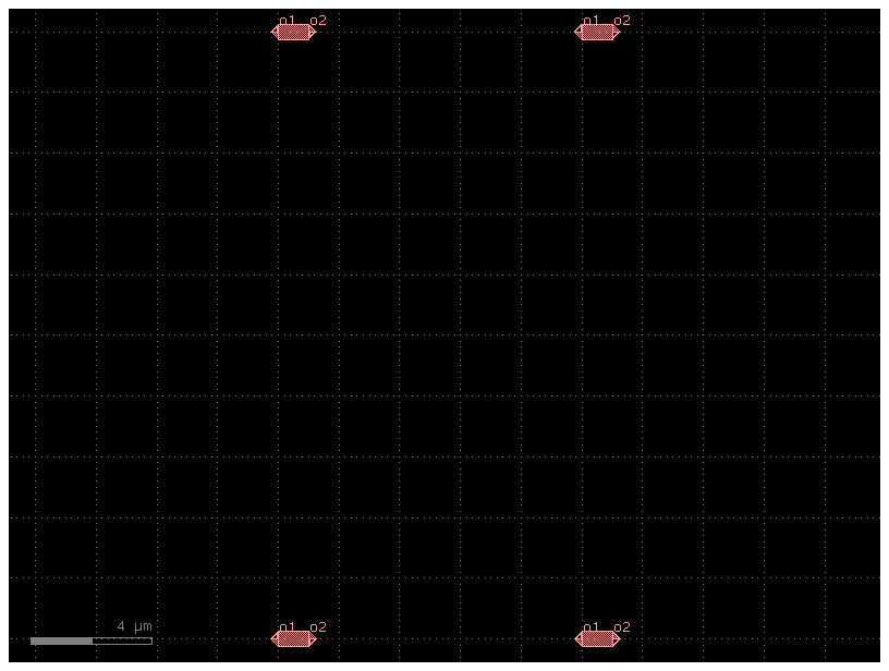
In GDS, there’s a type of structure called an “Instance” which takes a cell and repeats it NxM times on a fixed grid spacing. For convenience, Component includes this functionality with the add_ref() function.

Let’s make a new Component and put a big array of our Component c in it:

import gdsfactory as gf

c3 = gf.Component() 
c = gf.components.straight(length=1)

# This is the key step where the array is created.
# The add_ref function is used to place the unit cell c into the main component c3, but with additional parameters to create a grid:
# columns=2, rows=2: This specifies a 2x2 grid.
# column_pitch=10: The horizontal distance between the centers of adjacent columns is 10 µm.
# row_pitch=20: The vertical distance between the centers of adjacent rows is 20 µm.
# The variable aref holds a reference to this entire array.
aref = c3.add_ref(c, columns=2, rows=2, column_pitch=10, row_pitch=20)  
c3.add_ports(aref.ports) # The ports are then automatically named to indicate the position in the array (o1_0_0, o2_0_0, o1_1_0, o2_1_0, etc.).

# Reference the Component "c" 4 references in it with a 2 rows, 2 columns array.
c3.pprint_ports()
c3.draw_ports()
c3

┏━━━━━━┳━━━━━━━┳━━━━━━━━━━━━━┳━━━━━━━━━━┳━━━━━━━━━━━━━━┳━━━━━━━━━━━┓
┃ name ┃ width ┃ orientation ┃ layer    ┃ center       ┃ port_type ┃
┡━━━━━━╇━━━━━━━╇━━━━━━━━━━━━━╇━━━━━━━━━━╇━━━━━━━━━━━━━━╇━━━━━━━━━━━┩
│ o1   │ 0.5   │ 180.0       │ WG (1/0) │ (0.0, 0.0)   │ optical   │
│ o2   │ 0.5   │ 0.0         │ WG (1/0) │ (1.0, 0.0)   │ optical   │
│ o1   │ 0.5   │ 180.0       │ WG (1/0) │ (0.0, 20.0)  │ optical   │
│ o2   │ 0.5   │ 0.0         │ WG (1/0) │ (1.0, 20.0)  │ optical   │
│ o1   │ 0.5   │ 180.0       │ WG (1/0) │ (10.0, 0.0)  │ optical   │
│ o2   │ 0.5   │ 0.0         │ WG (1/0) │ (11.0, 0.0)  │ optical   │
│ o1   │ 0.5   │ 180.0       │ WG (1/0) │ (10.0, 20.0) │ optical   │
│ o2   │ 0.5   │ 0.0         │ WG (1/0) │ (11.0, 20.0) │ optical   │
└──────┴───────┴─────────────┴──────────┴──────────────┴───────────┘

aref['o1', 1, 1].x

10.0

aref.ports['o1', 0, 0].x

0.0

len(aref.ports)

8

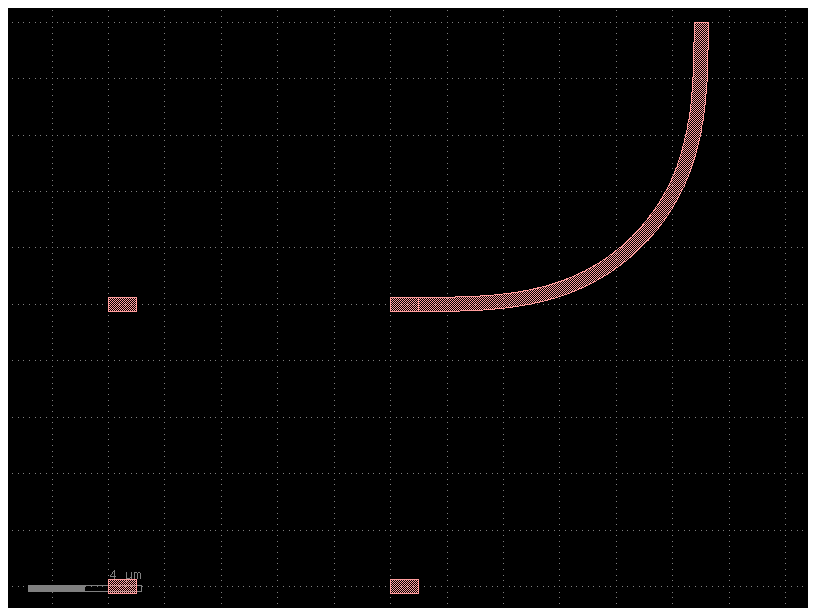
You can access the port from the array. Where (0, 0) is the bottom left instance in the array.

c = gf.Component()
b = c << gf.components.bend_euler()
s = c.add_ref(
    gf.components.straight(length=1),
    rows=2,
    row_pitch=10,
    columns=2,
    column_pitch=10,
)
b.connect("o1", s["o2", 1, 1])
c

gdsfactory provides you with similar functionality in gf.components.array. Notice that the port naming is different!

c4 = gf.Component()
c = gf.components.straight(length=1)
aref = c4 << gf.components.array(component=c, columns=2, rows=2, row_pitch=10, column_pitch=10)
c4.add_ports(aref.ports)
c4.pprint_ports()
c4.show()

┏━━━━━━━━┳━━━━━━━┳━━━━━━━━━━━━━┳━━━━━━━━━━┳━━━━━━━━━━━━━━┳━━━━━━━━━━━┓
┃ name   ┃ width ┃ orientation ┃ layer    ┃ center       ┃ port_type ┃
┡━━━━━━━━╇━━━━━━━╇━━━━━━━━━━━━━╇━━━━━━━━━━╇━━━━━━━━━━━━━━╇━━━━━━━━━━━┩
│ o1_1_1 │ 0.5   │ 180.0       │ WG (1/0) │ (0.0, 0.0)   │ optical   │
│ o2_1_1 │ 0.5   │ 0.0         │ WG (1/0) │ (1.0, 0.0)   │ optical   │
│ o1_2_1 │ 0.5   │ 180.0       │ WG (1/0) │ (0.0, 10.0)  │ optical   │
│ o2_2_1 │ 0.5   │ 0.0         │ WG (1/0) │ (1.0, 10.0)  │ optical   │
│ o1_1_2 │ 0.5   │ 180.0       │ WG (1/0) │ (10.0, 0.0)  │ optical   │
│ o2_1_2 │ 0.5   │ 0.0         │ WG (1/0) │ (11.0, 0.0)  │ optical   │
│ o1_2_2 │ 0.5   │ 180.0       │ WG (1/0) │ (10.0, 10.0) │ optical   │
│ o2_2_2 │ 0.5   │ 0.0         │ WG (1/0) │ (11.0, 10.0) │ optical   │
└────────┴───────┴─────────────┴──────────┴──────────────┴───────────┘

2025-10-29 02:38:51.578 | WARNING  | kfactory.kcell:show:4022 - Could not connect to klive server

help(gf.components.array)

Help on function array in module gdsfactory.components.containers.array_component:

array(component: 'ComponentSpec' = 'pad', columns: 'int' = 6, rows: 'int' = 1, column_pitch: 'float' = 150, row_pitch: 'float' = 150, add_ports: 'bool' = True, size: 'Size | None' = None, centered: 'bool' = False, post_process: 'PostProcesses | None' = None, auto_rename_ports: 'bool' = False) -> 'Component'
    Returns an array of components.
    
    Args:
        component: to replicate.
        columns: in x.
        rows: in y.
        column_pitch: pitch between columns.
        row_pitch: pitch between rows.
        auto_rename_ports: True to auto rename ports.
        add_ports: add ports from component into the array.
        size: Optional x, y size. Overrides columns and rows.
        centered: center the array around the origin.
        post_process: function to apply to the array after creation.
    
    Raises:
        ValueError: If columns > 1 and spacing[0] = 0.
        ValueError: If rows > 1 and spacing[1] = 0.
    
    .. code::
    
        2 rows x 4 columns
    
          column_pitch
          <---------->
         ___        ___       ___        ___
        |   |      |   |     |   |      |   |
        |___|      |___|     |___|      |___|
    
         ___        ___       ___        ___
        |   |      |   |     |   |      |   |
        |___|      |___|     |___|      |___|

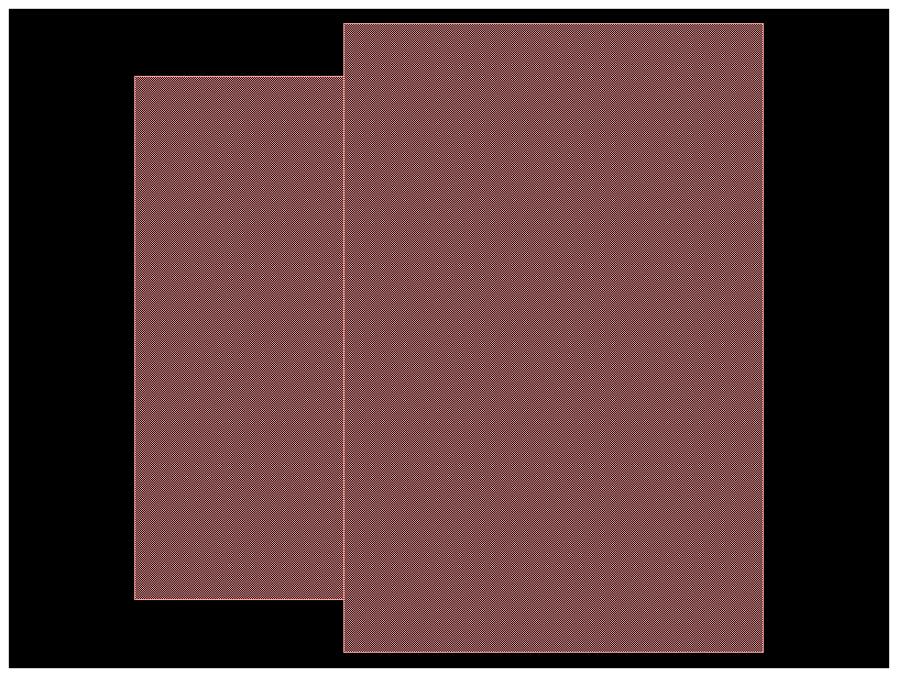
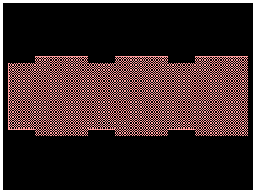
You can also create an array of references for periodic structures. Let us create a Distributed Bragg Reflector.

@gf.cell
def dbr_period(w1=0.5, w2=0.6, l1=0.2, l2=0.4, straight=gf.components.straight):
    """Return one DBR period."""
    c = gf.Component()
    r1 = c << straight(length=l1, width=w1)
    r2 = c << straight(length=l2, width=w2)

    # The second waveguide (r2) is automatically moved to connect its input port (o1) to the output port of the first waveguide (r1.ports["o2"]).
    # The allow_width_mismatch=True is necessary because the two waveguides have different widths.
    r2.connect(port="o1", other=r1.ports["o2"], allow_width_mismatch=True)
    
    # The unconnected input of the first section and the unconnected output of the second section are "exported".
    # These will become the ports of the main dbr_period component.
    c.add_port("o1", port=r1.ports["o1"])
    c.add_port("o2", port=r2.ports["o2"])
    return c


l1 = 0.2
l2 = 0.4
n = 3
period = dbr_period(l1=l1, l2=l2)
period

# period: The component to be repeated.
# columns=n: Creates n copies in the horizontal direction (since n was set to 3, it creates 3 copies).
# rows=1: Creates a single row.
# column_pitch=l1 + l2: This sets the horizontal distance between the start of each repeated period. 
# By setting it to the total length of one period (l1 + l2), the copies are placed perfectly end-to-end, creating a continuous structure.

dbr = gf.Component()
dbr.add_ref(period, columns=n, rows=1, column_pitch=l1 + l2)
dbr

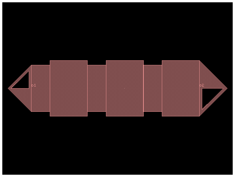
Finally we need to add ports to the new component.

# This adds two ports, o1 and o2, to the dbr component. However, it uses the ports from the single period component as a template. This means that initially:
# Port o1 is correctly placed at the start (0, 0).
# Port o2 is incorrectly placed at the end of the first period, not at the end of the whole 3-period structure.

p0 = dbr.add_port("o1", port=period.ports["o1"])
p1 = dbr.add_port("o2", port=period.ports["o2"])

# The crucial step that corrects the position of the output port (p1).
# (l1 + l2) * n: This calculates the total length of the DBR (the length of one period multiplied by the number of periods, n=3).
# By setting p1.dcenter to this new coordinate, the output port is moved to the very end of the final DBR structure.

p1.dcenter = ((l1 + l2) * n, 0)
dbr.draw_ports()
dbr

Connect references

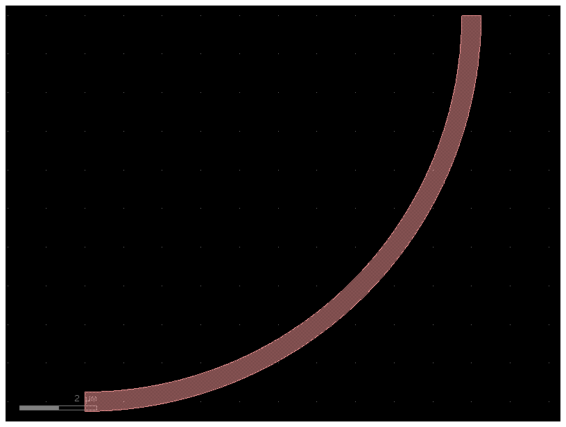
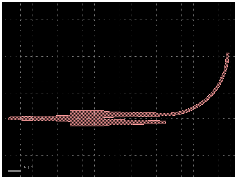
We have seen that once you create a reference you can manipulate the reference to move it to a location. Here we are going to connect that reference to a port. Remember that we follow that a certain reference source connects to a destination port.

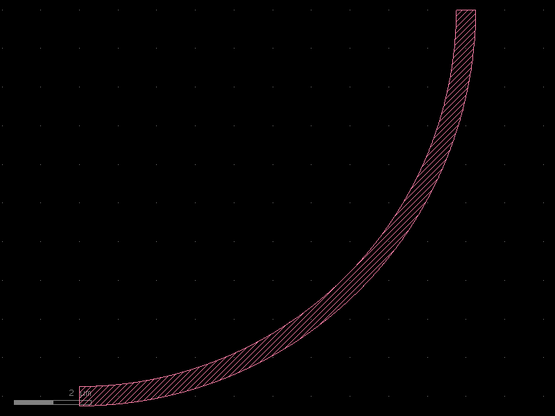
bend = gf.components.bend_circular()
bend

c = gf.Component()

mmi = c << gf.components.mmi1x2()
b = c << gf.components.bend_circular()
b.connect("o1", other=mmi.ports["o2"])

c.add_port("o1", port=mmi.ports["o1"])
c.add_port("o2", port=b.ports["o2"])
c.add_port("o3", port=mmi.ports["o3"])
c.plot()

You can also access the ports as reference[port_name] instead of reference.ports[port_name].

c = gf.Component()

mmi = c << gf.components.mmi1x2()
b = c << gf.components.bend_circular()
b.connect("o1", other=mmi["o2"])

#The unconnected ports of the sub-components are "exported" to become the ports of the main component c.
# c.add_port("o1", ...): The main input is the MMI's input port.
# c.add_port("o2", ...): The first main output is the bend's output port.
# c.add_port("o3", ...): The second main output is the MMI's other, still unconnected, output port (mmi["o3"]).
c.add_port("o1", port=mmi["o1"])
c.add_port("o2", port=b["o2"])
c.add_port("o3", port=mmi["o3"])
c.plot()

Notice that connect merges two ports together and does not imply that ports will remain connected.

Accessing parent cell from instances

You can access the cell from the instance.

print(b.cell.name)

bend_circular_gdsfactorypcomponentspbendspbend_circular_949aafe9

Accessing components from layout

You can also access the Component from the layout by the Component name. You can access the cells from the KCLayout:

bend = c.kcl[b.cell.name]
print(type(bend))
bend

<class 'kfactory.kcell.KCell'>

Port

You can assign custom names to ports and later rename them using gf.port.auto_rename_ports(prefix='o') or component.auto_rename_ports() which will rename them in place.

By default, ports are numbered clockwise starting from the bottom-left corner. The naming conventions are:

• Optical ports use the prefix o.

• Electrical ports use the prefix e.

Here is the default one we use (clockwise starting from bottom left corner):

             3   4
             |___|_
         2 -|      |- 5
            |      |
         1 -|______|- 6
             |   |
             8   7

Port names are defined in the gdsfactory.cross_section. For example:

• gdsfactory.cross_section.strip assigns o1 for the input and o2 for the output.

• gdsfactory.cross_section.metal1 assigns e1 for the input and e2 for the output.

Here are the most commonly used port types:

Port Type	Description
optical	Optical ports
electrical	Electrical ports
placement	Placement ports (excluded in netlist extraction)
vertical_te	For grating couplers with TE polarization
vertical_tm	For grating couplers with TM polarization
electrical_rf	Electrical ports for RF (high frequency)
pad	For pads
pad_rf	For RF pads
bump	For bumps
edge_coupler	For edge couplers

If you want to define another type that is not included you can do it like this:

gf.CONF.port_types += ["my_own_port_type"]

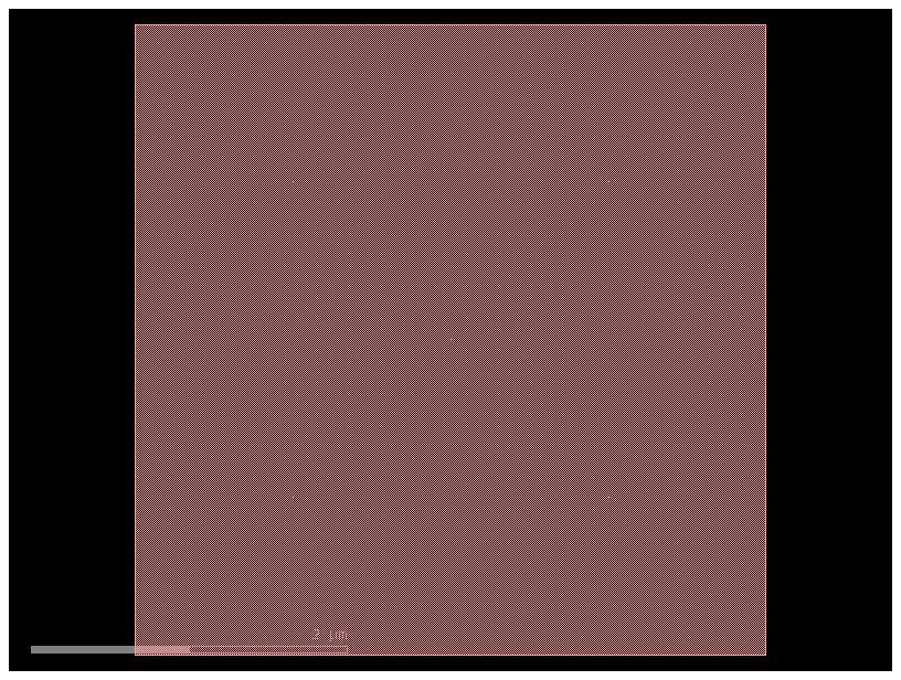
size = 4

# The gf.components.nxn function is a convenient tool for creating a rectangular component with a specified number of ports on each side.
c = gf.components.nxn(west=2, south=2, north=2, east=2, xsize=size, ysize=size)
c.plot()

c.pprint_ports()

┏━━━━━━┳━━━━━━━┳━━━━━━━━━━━━━┳━━━━━━━━━━┳━━━━━━━━━━━━━┳━━━━━━━━━━━┓
┃ name ┃ width ┃ orientation ┃ layer    ┃ center      ┃ port_type ┃
┡━━━━━━╇━━━━━━━╇━━━━━━━━━━━━━╇━━━━━━━━━━╇━━━━━━━━━━━━━╇━━━━━━━━━━━┩
│ o1   │ 0.5   │ 180.0       │ WG (1/0) │ (0.0, 1.25) │ optical   │
│ o2   │ 0.5   │ 180.0       │ WG (1/0) │ (0.0, 2.75) │ optical   │
│ o6   │ 0.5   │ 0.0         │ WG (1/0) │ (4.0, 1.25) │ optical   │
│ o5   │ 0.5   │ 0.0         │ WG (1/0) │ (4.0, 2.75) │ optical   │
│ o3   │ 0.5   │ 90.0        │ WG (1/0) │ (1.25, 4.0) │ optical   │
│ o4   │ 0.5   │ 90.0        │ WG (1/0) │ (2.75, 4.0) │ optical   │
│ o8   │ 0.5   │ 270.0       │ WG (1/0) │ (1.25, 0.0) │ optical   │
│ o7   │ 0.5   │ 270.0       │ WG (1/0) │ (2.75, 0.0) │ optical   │
└──────┴───────┴─────────────┴──────────┴─────────────┴───────────┘

You can get the optical ports by layer:

c.get_ports_list(layer=(1, 0))

[DPort(self.name='o1', self.width=0.5, trans=r180 *1 0,1.25, layer=WG (1/0), port_type=optical),
 DPort(self.name='o2', self.width=0.5, trans=r180 *1 0,2.75, layer=WG (1/0), port_type=optical),
 DPort(self.name='o6', self.width=0.5, trans=r0 *1 4,1.25, layer=WG (1/0), port_type=optical),
 DPort(self.name='o5', self.width=0.5, trans=r0 *1 4,2.75, layer=WG (1/0), port_type=optical),
 DPort(self.name='o3', self.width=0.5, trans=r90 *1 1.25,4, layer=WG (1/0), port_type=optical),
 DPort(self.name='o4', self.width=0.5, trans=r90 *1 2.75,4, layer=WG (1/0), port_type=optical),
 DPort(self.name='o8', self.width=0.5, trans=r270 *1 1.25,0, layer=WG (1/0), port_type=optical),
 DPort(self.name='o7', self.width=0.5, trans=r270 *1 2.75,0, layer=WG (1/0), port_type=optical)]

c.pprint_ports(layer=(1, 0))

┏━━━━━━┳━━━━━━━┳━━━━━━━━━━━━━┳━━━━━━━━━━┳━━━━━━━━━━━━━┳━━━━━━━━━━━┓
┃ name ┃ width ┃ orientation ┃ layer    ┃ center      ┃ port_type ┃
┡━━━━━━╇━━━━━━━╇━━━━━━━━━━━━━╇━━━━━━━━━━╇━━━━━━━━━━━━━╇━━━━━━━━━━━┩
│ o1   │ 0.5   │ 180.0       │ WG (1/0) │ (0.0, 1.25) │ optical   │
│ o2   │ 0.5   │ 180.0       │ WG (1/0) │ (0.0, 2.75) │ optical   │
│ o6   │ 0.5   │ 0.0         │ WG (1/0) │ (4.0, 1.25) │ optical   │
│ o5   │ 0.5   │ 0.0         │ WG (1/0) │ (4.0, 2.75) │ optical   │
│ o3   │ 0.5   │ 90.0        │ WG (1/0) │ (1.25, 4.0) │ optical   │
│ o4   │ 0.5   │ 90.0        │ WG (1/0) │ (2.75, 4.0) │ optical   │
│ o8   │ 0.5   │ 270.0       │ WG (1/0) │ (1.25, 0.0) │ optical   │
│ o7   │ 0.5   │ 270.0       │ WG (1/0) │ (2.75, 0.0) │ optical   │
└──────┴───────┴─────────────┴──────────┴─────────────┴───────────┘

or by width:

c.get_ports_list(width=500)

[]

# A straight_heater_metal component is created. 
# This is a complex component that has both optical ports for the waveguide and electrical ports for the metal heater.
c0 = gf.components.straight_heater_metal()
c0.pprint_ports() # This command prints a neatly formatted table of the ports on the original component, c0. 

┏━━━━━━┳━━━━━━━┳━━━━━━━━━━━━━┳━━━━━━━━━━━┳━━━━━━━━━━━━━━━━━━━━━━━━━━━━┳━━━━━━━━━━━━┓
┃ name ┃ width ┃ orientation ┃ layer     ┃ center                     ┃ port_type  ┃
┡━━━━━━╇━━━━━━━╇━━━━━━━━━━━━━╇━━━━━━━━━━━╇━━━━━━━━━━━━━━━━━━━━━━━━━━━━╇━━━━━━━━━━━━┩
│ o1   │ 0.5   │ 180.0       │ WG (1/0)  │ (0.0, 0.0)                 │ optical    │
│ o2   │ 0.5   │ 0.0         │ WG (1/0)  │ (320.0, 0.0)               │ optical    │
│ l_e1 │ 11.0  │ 180.0       │ M3 (49/0) │ (-15.9, 0.0)               │ electrical │
│ l_e2 │ 11.0  │ 90.0        │ M3 (49/0) │ (-10.4, 5.5)               │ electrical │
│ l_e3 │ 11.0  │ 0.0         │ M3 (49/0) │ (-4.9, 0.0)                │ electrical │
│ l_e4 │ 11.0  │ 270.0       │ M3 (49/0) │ (-10.4, -5.5)              │ electrical │
│ r_e1 │ 11.0  │ 180.0       │ M3 (49/0) │ (324.90000000000003, 0.0)  │ electrical │
│ r_e2 │ 11.0  │ 90.0        │ M3 (49/0) │ (330.40000000000003, 5.5)  │ electrical │
│ r_e3 │ 11.0  │ 0.0         │ M3 (49/0) │ (335.90000000000003, 0.0)  │ electrical │
│ r_e4 │ 11.0  │ 270.0       │ M3 (49/0) │ (330.40000000000003, -5.5) │ electrical │
└──────┴───────┴─────────────┴───────────┴────────────────────────────┴────────────┘

c1 = c0.dup() # A duplicate of the component is created and stored in c1. Then, the auto_rename_ports() function is called on this new component.
c1.auto_rename_ports()
c1.pprint_ports()

┏━━━━━━┳━━━━━━━┳━━━━━━━━━━━━━┳━━━━━━━━━━━┳━━━━━━━━━━━━━━━━━━━━━━━━━━━━┳━━━━━━━━━━━━┓
┃ name ┃ width ┃ orientation ┃ layer     ┃ center                     ┃ port_type  ┃
┡━━━━━━╇━━━━━━━╇━━━━━━━━━━━━━╇━━━━━━━━━━━╇━━━━━━━━━━━━━━━━━━━━━━━━━━━━╇━━━━━━━━━━━━┩
│ o1   │ 0.5   │ 180.0       │ WG (1/0)  │ (0.0, 0.0)                 │ optical    │
│ o2   │ 0.5   │ 0.0         │ WG (1/0)  │ (320.0, 0.0)               │ optical    │
│ e1   │ 11.0  │ 180.0       │ M3 (49/0) │ (-15.9, 0.0)               │ electrical │
│ e3   │ 11.0  │ 90.0        │ M3 (49/0) │ (-10.4, 5.5)               │ electrical │
│ e6   │ 11.0  │ 0.0         │ M3 (49/0) │ (-4.9, 0.0)                │ electrical │
│ e8   │ 11.0  │ 270.0       │ M3 (49/0) │ (-10.4, -5.5)              │ electrical │
│ e2   │ 11.0  │ 180.0       │ M3 (49/0) │ (324.90000000000003, 0.0)  │ electrical │
│ e4   │ 11.0  │ 90.0        │ M3 (49/0) │ (330.40000000000003, 5.5)  │ electrical │
│ e5   │ 11.0  │ 0.0         │ M3 (49/0) │ (335.90000000000003, 0.0)  │ electrical │
│ e7   │ 11.0  │ 270.0       │ M3 (49/0) │ (330.40000000000003, -5.5) │ electrical │
└──────┴───────┴─────────────┴───────────┴────────────────────────────┴────────────┘

You can also rename them with a different port naming convention:

• Prefix: add e for electrical o for optical

• Clockwise

• Counter-clockwise

• Orientation E East, W West, N North, S South

• Note: All ports are east facing by default and need to be rotated in order to have a different orientation.

Here is the default one we use (clockwise starting from bottom left west facing port):

             3   4
             |___|_
         2 -|      |- 5
            |      |
         1 -|______|- 6
             |   |
             8   7

c = gf.Component("demo_ports")
nxn = gf.components.nxn(west=2, north=2, east=2, south=2, xsize=4, ysize=4)
ref = c.add_ref(nxn)
c.add_ports(ref.ports)
c.plot()

gf.port.pprint_ports(ref.ports)

┏━━━━━━┳━━━━━━━┳━━━━━━━━━━━━━┳━━━━━━━━━━┳━━━━━━━━━━━━━┳━━━━━━━━━━━┓
┃ name ┃ width ┃ orientation ┃ layer    ┃ center      ┃ port_type ┃
┡━━━━━━╇━━━━━━━╇━━━━━━━━━━━━━╇━━━━━━━━━━╇━━━━━━━━━━━━━╇━━━━━━━━━━━┩
│ o1   │ 0.5   │ 180.0       │ WG (1/0) │ (0.0, 1.25) │ optical   │
│ o2   │ 0.5   │ 180.0       │ WG (1/0) │ (0.0, 2.75) │ optical   │
│ o6   │ 0.5   │ 0.0         │ WG (1/0) │ (4.0, 1.25) │ optical   │
│ o5   │ 0.5   │ 0.0         │ WG (1/0) │ (4.0, 2.75) │ optical   │
│ o3   │ 0.5   │ 90.0        │ WG (1/0) │ (1.25, 4.0) │ optical   │
│ o4   │ 0.5   │ 90.0        │ WG (1/0) │ (2.75, 4.0) │ optical   │
│ o8   │ 0.5   │ 270.0       │ WG (1/0) │ (1.25, 0.0) │ optical   │
│ o7   │ 0.5   │ 270.0       │ WG (1/0) │ (2.75, 0.0) │ optical   │
└──────┴───────┴─────────────┴──────────┴─────────────┴───────────┘

You can also get the ports counter-clockwise:

             4   3
             |___|_
         5 -|      |- 2
            |      |
         6 -|______|- 1
             |   |
             7   8

c.get_ports_list(clockwise=False)

[DPort(self.name='o1', self.width=0.5, trans=r180 *1 0,1.25, layer=WG (1/0), port_type=optical),
 DPort(self.name='o2', self.width=0.5, trans=r180 *1 0,2.75, layer=WG (1/0), port_type=optical),
 DPort(self.name='o6', self.width=0.5, trans=r0 *1 4,1.25, layer=WG (1/0), port_type=optical),
 DPort(self.name='o5', self.width=0.5, trans=r0 *1 4,2.75, layer=WG (1/0), port_type=optical),
 DPort(self.name='o3', self.width=0.5, trans=r90 *1 1.25,4, layer=WG (1/0), port_type=optical),
 DPort(self.name='o4', self.width=0.5, trans=r90 *1 2.75,4, layer=WG (1/0), port_type=optical),
 DPort(self.name='o8', self.width=0.5, trans=r270 *1 1.25,0, layer=WG (1/0), port_type=optical),
 DPort(self.name='o7', self.width=0.5, trans=r270 *1 2.75,0, layer=WG (1/0), port_type=optical)]

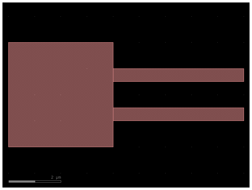
Lets extend the east facing ports (orientation = 0 deg):

import gdsfactory as gf

# This defines a standard strip waveguide cross-section, which contains information about the waveguide's width, layer, and other properties.
# A strip waveguide has a core with material which has a high refractive index, whereas the cladding (material surrounding the core) has a low refractive index.
# This contrast leads to the strip being able to confine light very tightly, thus allowing for sharp bends with minimal loss of light.
cross_section = gf.cross_section.strip()

# A 4x4 square component with two ports on each side is created. 
# The cross_section parameter ensures that all the ports on this component are defined as strip waveguides.
nxn = gf.components.nxn(
    west=2, north=2, east=2, south=2, xsize=4, ysize=4, cross_section=cross_section)

# The extend_ports function takes the nxn component and adds straight extensions to some of its ports.
# component=nxn: The component to modify.
# orientation=0: This tells the function to only add extensions to the ports that have an orientation of 0 degrees, 
# which corresponds to the ports on the east (right) side of the component.
c = gf.components.extension.extend_ports(component=nxn, orientation=0)
c.plot()

c.pprint_ports()

┏━━━━━━┳━━━━━━━┳━━━━━━━━━━━━━┳━━━━━━━━━━┳━━━━━━━━━━━━━┳━━━━━━━━━━━┓
┃ name ┃ width ┃ orientation ┃ layer    ┃ center      ┃ port_type ┃
┡━━━━━━╇━━━━━━━╇━━━━━━━━━━━━━╇━━━━━━━━━━╇━━━━━━━━━━━━━╇━━━━━━━━━━━┩
│ o1   │ 0.5   │ 180.0       │ WG (1/0) │ (0.0, 1.25) │ optical   │
│ o2   │ 0.5   │ 180.0       │ WG (1/0) │ (0.0, 2.75) │ optical   │
│ o6   │ 0.5   │ 0.0         │ WG (1/0) │ (9.0, 1.25) │ optical   │
│ o5   │ 0.5   │ 0.0         │ WG (1/0) │ (9.0, 2.75) │ optical   │
│ o3   │ 0.5   │ 90.0        │ WG (1/0) │ (1.25, 4.0) │ optical   │
│ o4   │ 0.5   │ 90.0        │ WG (1/0) │ (2.75, 4.0) │ optical   │
│ o8   │ 0.5   │ 270.0       │ WG (1/0) │ (1.25, 0.0) │ optical   │
│ o7   │ 0.5   │ 270.0       │ WG (1/0) │ (2.75, 0.0) │ optical   │
└──────┴───────┴─────────────┴──────────┴─────────────┴───────────┘

Port markers (Pins)

You can add pins (port markers) to each port. Different foundries do this differently, so gdsfactory supports all of them.

• Square with port inside the component.

• Square centered (half inside, half outside component).

• Triangular pointing towards the outside of the port.

• Path (SiEPIC).

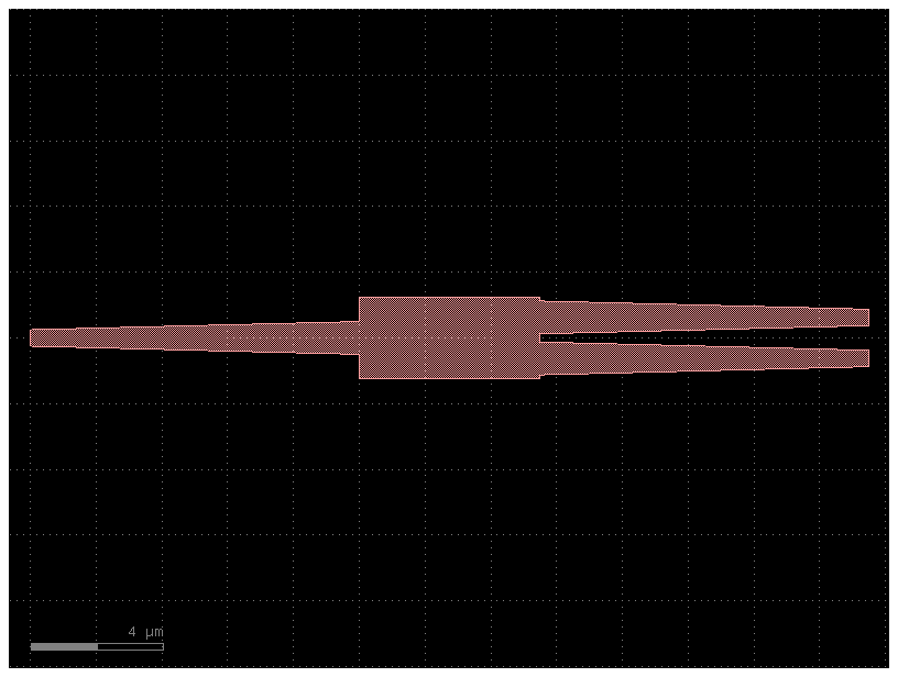
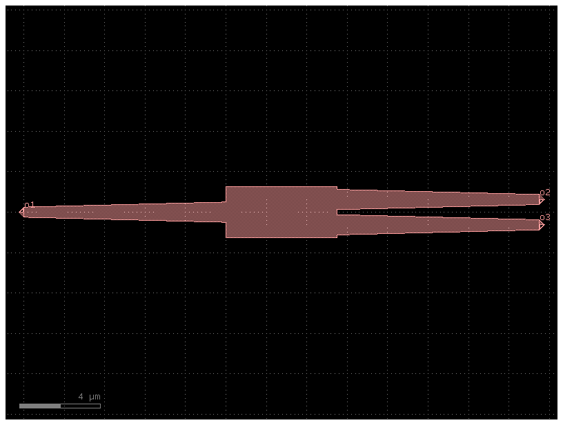
c = gf.components.mmi1x2()
c.plot()

c = gf.components.mmi1x2()

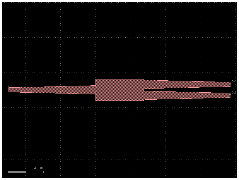
# The add_pins_container function takes the mmi component and returns a new component that includes the original MMI geometry plus visual annotations for each port. 
# These "pins" are typically short path markers and text labels showing the port's name (e.g., "o1"), making them easy to identify visually.
c_with_pins = gf.add_pins.add_pins_container(c)

# The plot will show the MMI component with a pin and a text label sticking out from each of its three ports, clearly indicating their location and name.
# This is a useful utility for debugging and inspecting component layouts.
c_with_pins.plot()

c = gf.components.mmi1x2()
c.draw_ports()
c.plot()

Component_sequence

When you have repetitive connections you can describe the connectivity as an ASCII map.

import gdsfactory as gf

# This creates a 180-degree circular bend, which is a U-shaped waveguide used to turn the path of light around completely.
bend180 = gf.components.bend_circular180() 

# The following function creates a straight waveguide with PIN junctions and heaters. It includes the central silicon waveguide, 
# doped regions (positive and negative), and metal contacts for applying a voltage, often used for thermal tuning or modulation.
# The straight_pin component is designed to be thermo-optic phase shifter, not just a simple waveguide.
# A thermo-optic phase shifter is a device on a photonic chip that uses heat to control the phase of a light wave.
wg_pin = gf.components.straight_pin(length=40)

# This creates a simple, standard straight waveguide, which is the most basic component for guiding light in a straight line.
wg = gf.components.straight()

# Define a map between symbols and (component, input port, output port).
symbol_to_component = {
    "D": (bend180, "o1", "o2"),
    "C": (bend180, "o2", "o1"),
    "P": (wg_pin, "o1", "o2"),
    "-": (wg, "o1", "o2"),
}

# Generate a sequence.
# This is simply a chain of characters. Each of them represents a component.
# with a given input and and a given output.

sequence = "DC-P-P-P-P-CD"
component = gf.components.component_sequence(

    # The symbol_to_component is a Python dictionary that acts as a key, mapping the symbols from the sequence string to actual gdsfactory components.
    sequence=sequence, symbol_to_component=symbol_to_component)
component.plot()

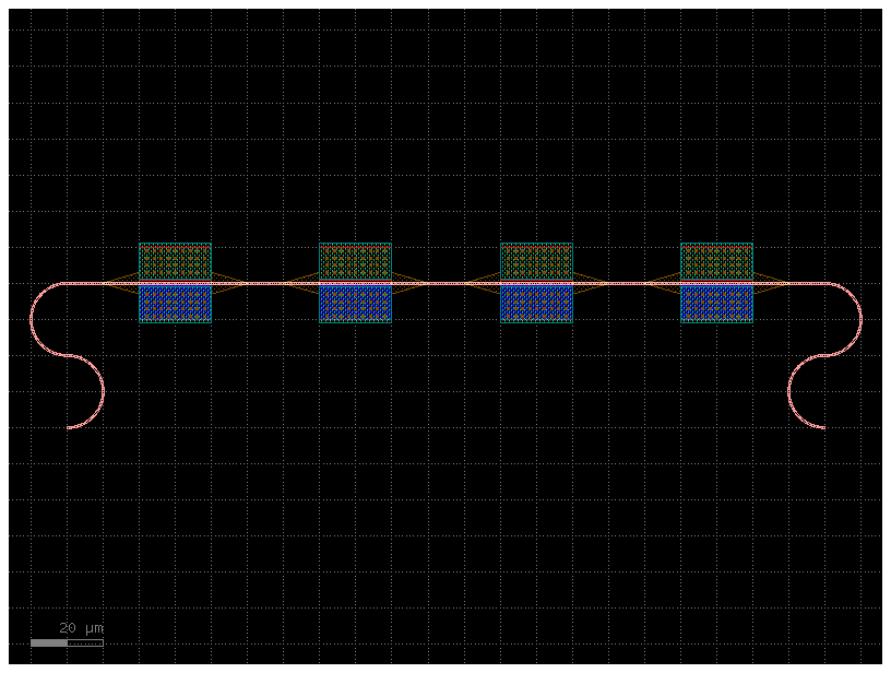
As the sequence is defined as a string you can use the string operations to easily build complex sequences

Movement

You can move, rotate and mirror Instance as well as Port, Polygon, Instance, Label, and Group

import gdsfactory as gf

# Start with a blank Component.
c = gf.Component()

# Create some more Components with shapes.
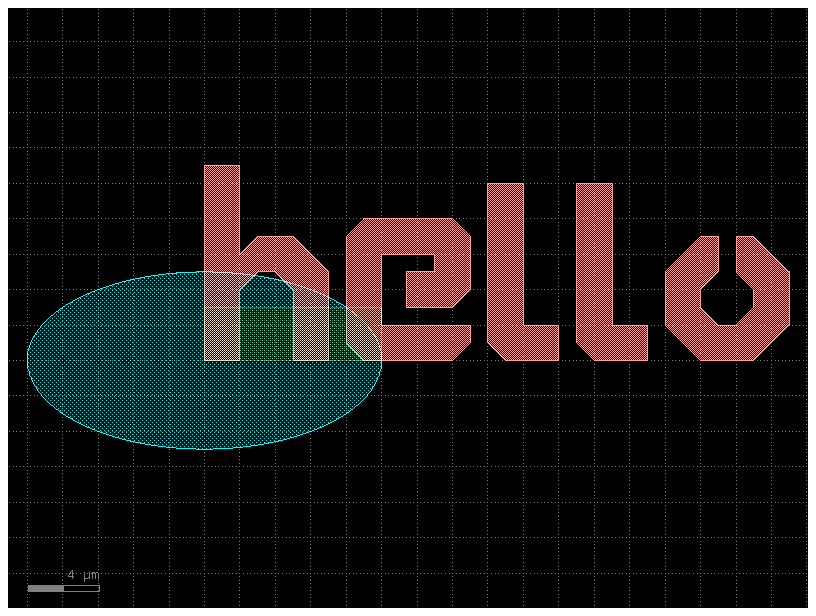
T = gf.components.text("hello", size=10, layer=(1, 0))
E = gf.components.ellipse(radii=(10, 5), layer=(2, 0))
R = gf.components.rectangle(size=(10, 3), layer=(3, 0))

# Add the shapes to c as instances.
text = c << T
ellipse = c << E
rect1 = c << R
rect2 = c << R

c.plot()

c = gf.Component()
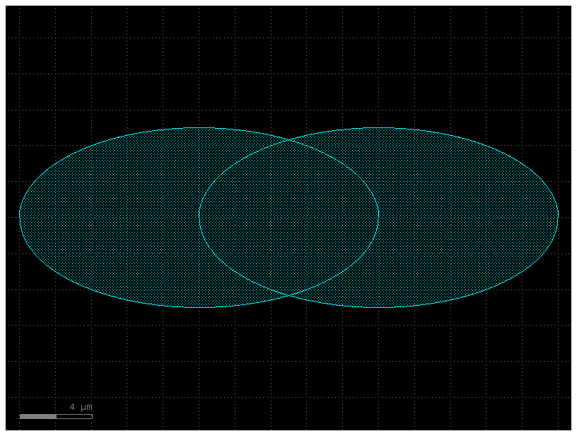
e1 = c << gf.components.ellipse(radii=(10, 5), layer=(2, 0))
e2 = c << gf.components.ellipse(radii=(10, 5), layer=(2, 0))
e1.movex(10)
c.plot()

c = gf.Component()
e1 = c << gf.components.ellipse(radii=(10, 5), layer=(2, 0))
e2 = c << gf.components.ellipse(radii=(10, 5), layer=(2, 0))

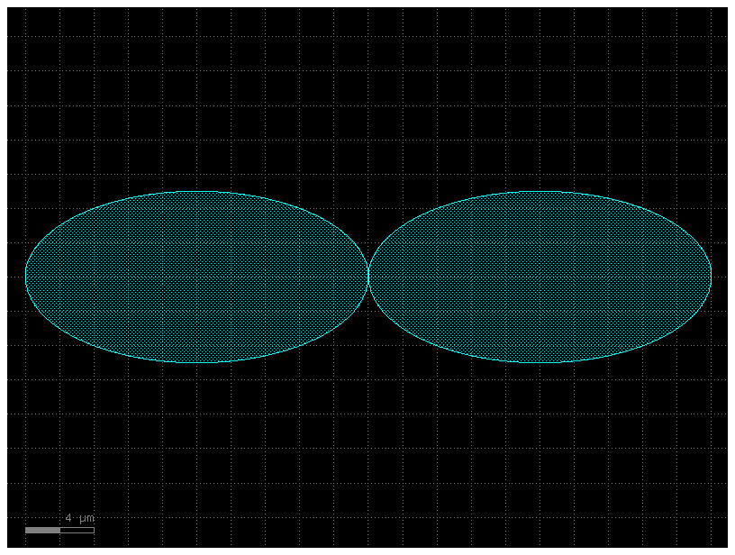
# This moves the second ellipse (e2) horizontally until its leftmost point (xmin) is perfectly aligned with the rightmost point (xmax) of the first ellipse (e1).
e2.xmin = e1.xmax
c.plot()

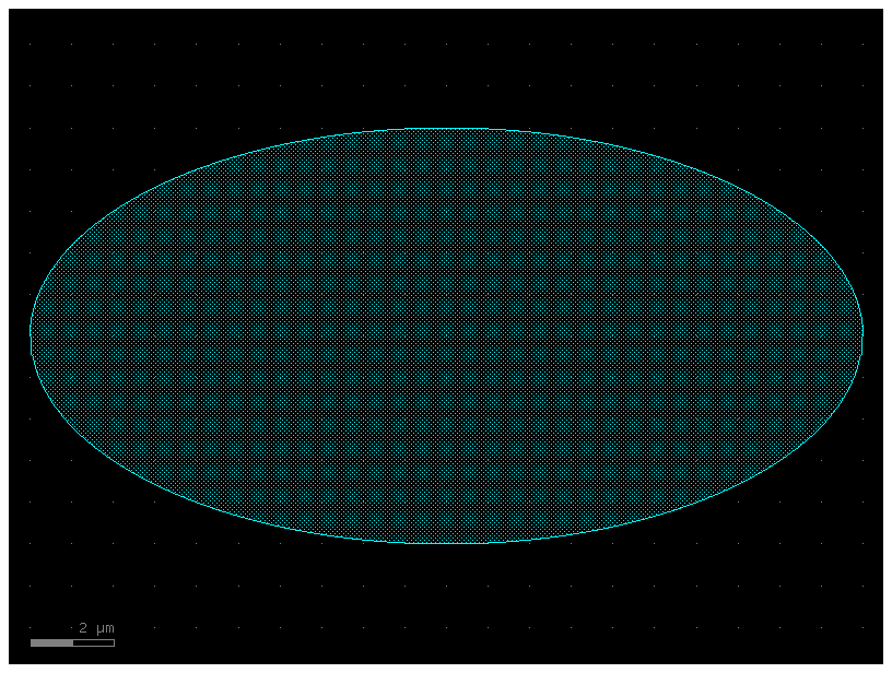
# Now you can practice move and rotate the objects.

c = gf.Component()
E = gf.components.ellipse(radii=(10, 5), layer=(2, 0))
e1 = c << E
e2 = c << E
c.plot()

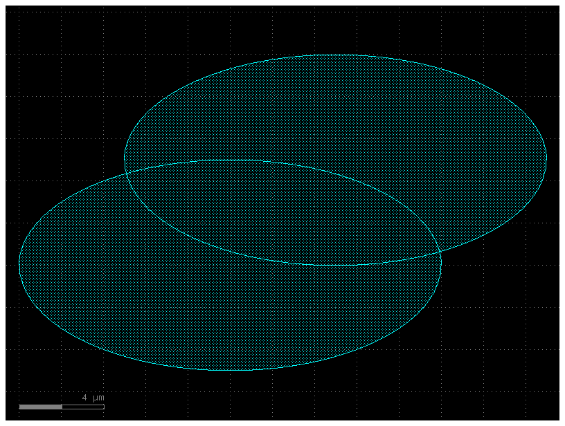
c = gf.Component()
e = gf.components.ellipse(radii=(10, 5), layer=(2, 0))
e1 = c << e
e2 = c << e
e2.move((5, 5))  # Translate by dx = 5, dy = 5
c.plot()

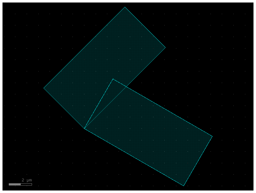
c = gf.Component()
r = gf.components.rectangle(size=(10, 5), layer=(2, 0))
rect1 = c << r
rect2 = c << r

rect1.rotate(45)  # Rotate the first straight by 45 degrees around (0,0).
rect2.rotate(-30)  # Rotate the second straight by -30 degrees around (1,1).
c.plot()

import gdsfactory as gf

c = gf.Component()
text = c << gf.components.text("hello")
text.dmirror(p1=(1, 1), p2=(1, 3))  
# Reflects across the line formed by p1 and p2.
c.plot()

c = gf.Component()
text = c << gf.components.text("hello")
c.plot()

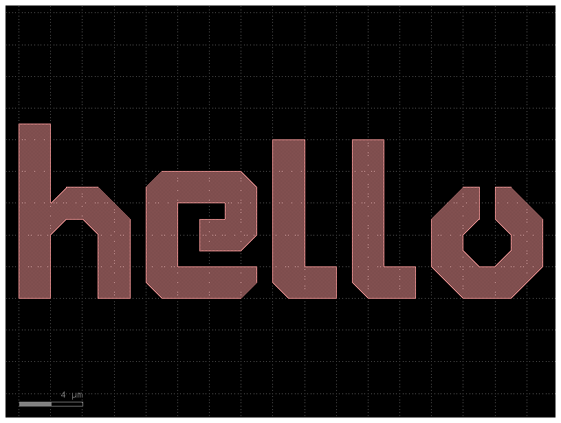
Each Component and Instance object has several properties which can be used to learn information about the object (for instance where it’s center coordinate is). Several of these properties can actually be used to move the geometry by assigning them new values.

Available properties are:

• xmin / xmax: minimum and maximum x-values of all points within the object

• ymin / ymax: minimum and maximum y-values of all points within the object

• x: centerpoint between minimum and maximum x-values of all points within the object

• y: centerpoint between minimum and maximum y-values of all points within the object

• bbox: bounding box (see note below) in format ((xmin,ymin),(xmax,ymax))

• center: center of bounding box

print(
    "printing the bounding box of text in terms of [(xmin, ymin), (xmax, ymax)] in um"
)
print(text.dbbox())  # In Decimal um (float).
print("xsize and ysize:")
print(text.xsize)  # Will print the width of text in the x dimension in um
print(text.ysize)  # Will print the height of text in the y dimension in um

print("center:")
print(text.dcenter)  # Gives you the center coordinate of its bounding box in DBU
print("xmax")
print(text.xmax)  # Gives you the rightmost (+x) edge of the text bounding box

printing the bounding box of text in terms of [(xmin, ymin), (xmax, ymax)] in um
(1,0;34,11)
xsize and ysize:
33.0
11.0
center:
(17.5, 5.5)
xmax
34.0

c = gf.Component()
text = c << gf.components.text("hello")
E = gf.components.ellipse(radii=(10, 5), layer=(3, 0))
R = gf.components.rectangle(size=(10, 5), layer=(2, 0))
rect1 = c << R
rect2 = c << R
ellipse = c << E
c.plot()

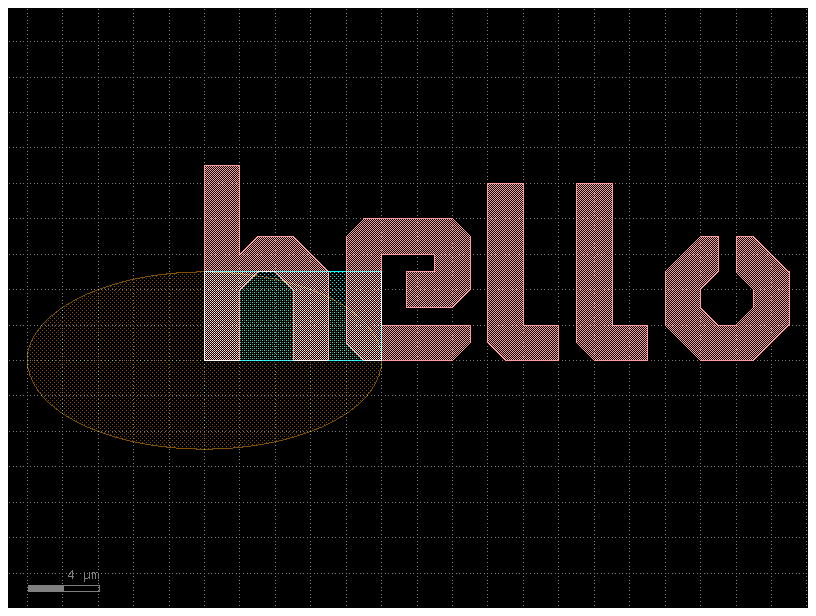
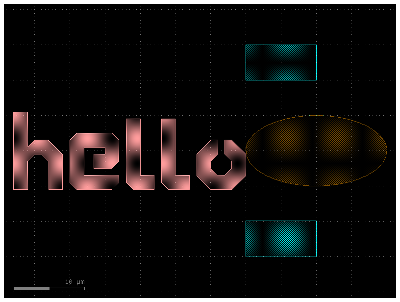
ellipse.dcenter = (0, 0)  # Move the ellipse to the center of the bounding box.

# Next, let us move the text to the left edge of the ellipse.
text.y = (
    ellipse.y
)  # Move the text so that its y-center is equal to the y-center of the ellipse.
text.xmax = ellipse.xmin  # Moves the ellipse so its xmax == the ellipse's xmin.

# Align the right edge of the rectangles with the x=0 axis.
rect1.xmax = 0
rect2.xmax = 0

# Move the rectangles above and below the ellipse.
rect1.ymin = ellipse.ymax + 5
rect2.ymax = ellipse.ymin - 5

c.plot()

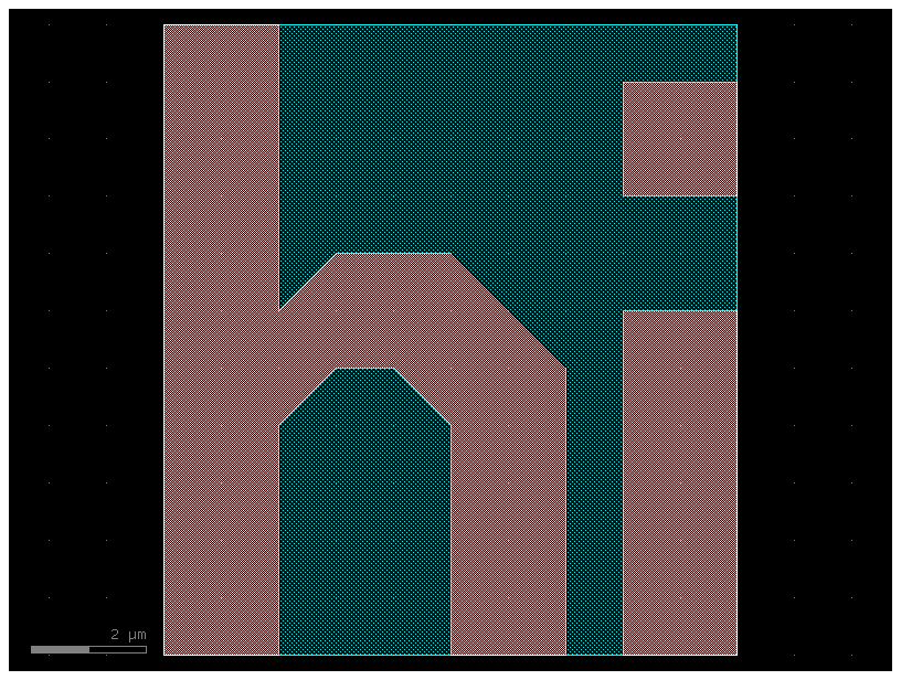
import gdsfactory as gf

# A bounding box is the smallest enclosing box which contains all points of the geometry.

c = gf.Component()
text = c << gf.components.text("hi")
c << gf.components.bbox(text, layer=(2, 0))
fig = c.plot()

c = gf.Component()
text = c << gf.components.text("bye")
device_bbox = text.bbox

# The gf.get_padding_points function takes the text component as input and calculates the vertices of a new polygon that surrounds it.
# default=1: This specifies a uniform padding of 1 µm on all sides.
# The resulting list of points is then used to add a new polygon to the component c on a different layer, (2, 0).
c.add_polygon(gf.get_padding_points(text, default=1), layer=(2, 0))
c.plot()

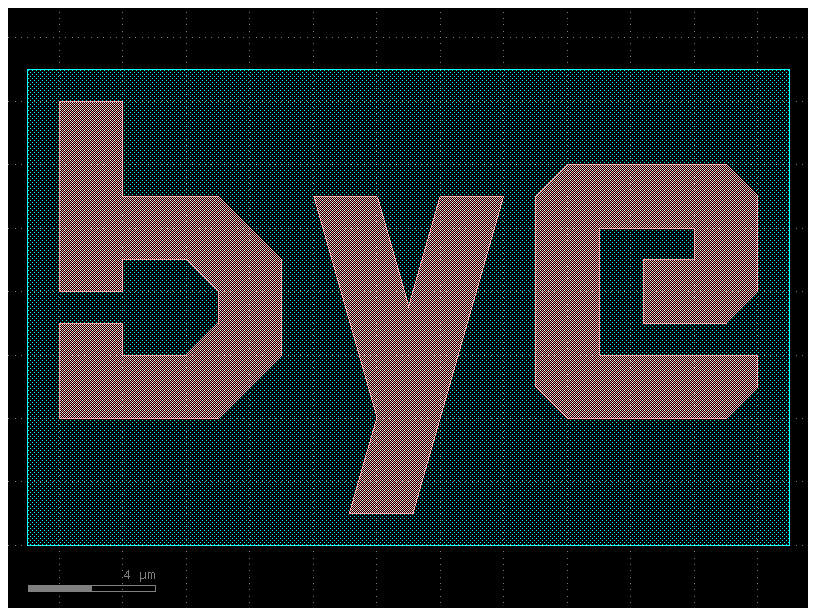
# When we query the properties of c, they will be calculated with respect to this bounding-rectangle.  For instance:

print("Center of Component c:")
print(c.dcenter)

print("X-max of Component c:")
print(c.xmax)

Center of Component c:
(12.0, 3.5)
X-max of Component c:
24.0

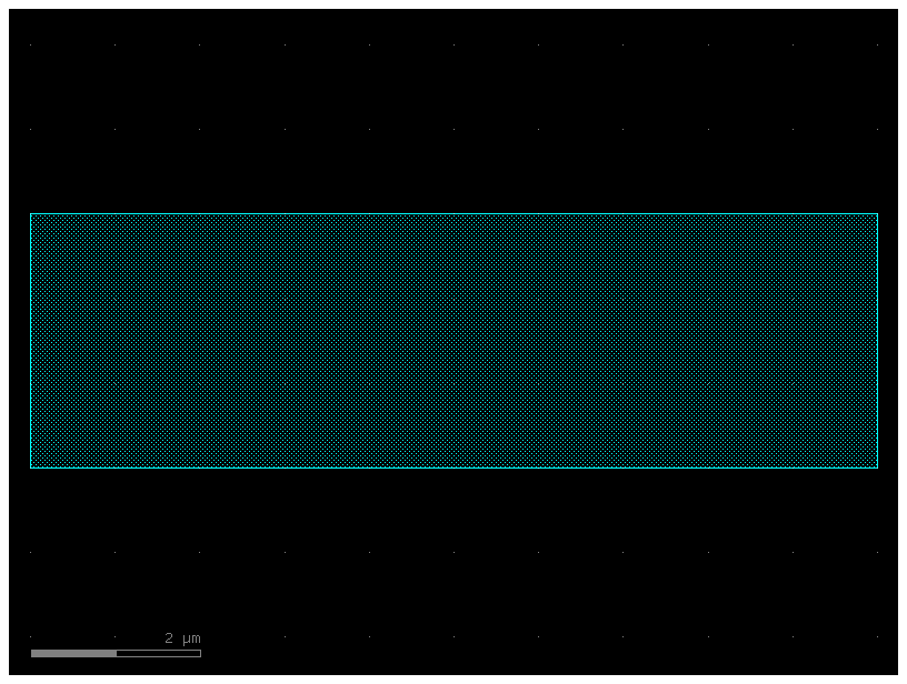
c = gf.Component()
R = gf.components.rectangle(size=(10, 3), layer=(2, 0))
rect1 = c << R
f = c.plot()

# You can chain many of the movement/manipulation functions because they all return the object they manipulate.
# For instance you can combine two expressions:

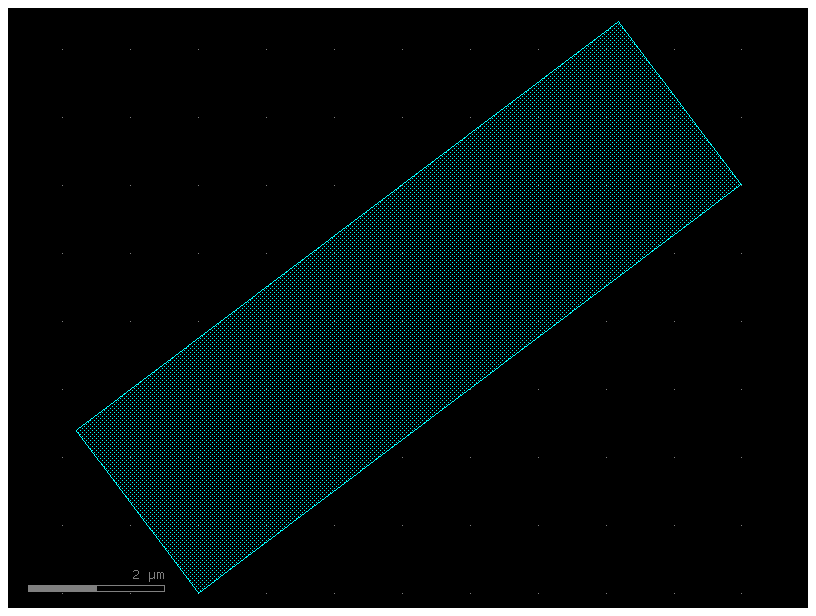
rect1.rotate(angle=37)
rect1.move((10, 20))
f = c.plot()

# ...into this single-line expression:

c = gf.Component()
R = gf.components.rectangle(size=(10, 3), layer=(2, 0))
rect1 = c << R
rect1.rotate(angle=37).move((10, 20))
f = c.plot()